Typology and Problematics of Fixed Notation for the Representation of Electroacoustic and Digital Media

Preamble; Part I. Waveform display notation

by jef chippewa

This is the first in a series of texts dealing with the topic of notation of electroacoustic and digital media. Following the present discussion of Waveform Display Notation, subsequent parts will address other types of notation as well as broader issues related to the use of notation in electroacoustic practices: Sonogramme; Graphic Representation and Spectromorphology; Animated Notation; Text Notation; Traditional and Proportional Notation; Considerations of Score Format and Function.

Preamble

The intention of this text is neither to discuss what constitutes an electroacoustic work nor to reinforce or blur the boundaries that delineate to varying degrees a diverse range of æsthetic approaches to sound-based artistic creation. The term “electroacoustic” is therefore understood and used here to refer to the broader category of creative practices concerned with the production and/or performance of abstract works generally intended as “concert music” for which some form of electronic means is employed in the generation, manipulation or control of sound, either during the creative stages, in the studio or in a live performance context. Moreover, the live performance of the work may involve “fixed” sound that can be interpreted in different manners in different performances, or may involve the production of new materials at each instance using an algorithmic, generative or improvisational approach.

To this end, the term “electroacoustic” is understood to encompass, but not be limited to:

• Acousmatic, soundscape, musique concrète and radiophonic practices;
• Tape music, fixed media, electronic music and synthesized sound;
• Live electronics and various forms of live or pre-recorded MIDI-generated sound;
• Sound generated and/or processed by Max/MSP, PD, Supercollider or other such audio software;
• Other practices that may have unintentionally been overlooked in this discussion.

A “mixed” work is then one that features one or more of these media in conjunction with one or more acoustic or hybrid acoustic-electronic instruments that may have or be characterized by a more traditional performance paradigm.

In the present context we are concerned purely with the visual representation — some form of sonic or musical notation — of these practices in one or more symbolic and/or graphic forms. The discussion will remain restricted to those electroacoustic works and practices for which some aspect is predetermined and the “same” in different performances (even if some of it is to be improvised) and which therefore require a degree of fixed notation, or visualization, to represent them. This visual representation might illustrate what is meant to be played or heard at a given moment in the work’s presentation, or it may indicate some stage or aspect of the work that has been documented either as reference or for later re-performance.

Each overview of the different methods of representing sound in electroacoustic practices (i.e. notation) includes a description of the salient characteristics of the notation type and a discussion of how well or poorly it is able to represent or show aspects of the sound such as frequency content, rhythm and texture, sound levels (dynamics), polyphony and layering of voices, similarities and dissimilarities of materials, and more. The discussion of each type of notation is augmented by examples in which the particular pros and cons are manifest, and, where relevant, some indications of how these problems can be resolved or how their inadequacies can be used to advantage in particular contexts.

Types of Notational Representation

The individual categories or types of notation are considered in this text as distinct and separate entities only for the purpose of clearly identifying their characteristics, and, more importantly, the advantages and disadvantages of their use for the representation of electroacoustic practices. However, there is no shortage of scores in which more than one form of notation is employed throughout or in different parts of the piece. Further, and again this diverges substantially from much of the notation of instrumental music, any combination of these notation types may be used concurrently, and the proportion of their use individually or even their presence altogether may change according to the local and regional needs of the piece. In the case of mixed works, depending on the type of music involved and how the two parts (acoustic and electronic) are intended to converge in the performance, the notation of the instrumental part may or may not be notated in a similar manner as the full score or the electronic or digital sound component.

And it is important to emphasize that there is really no absolute “good” or “bad” when it comes to the question of artistic practice and the portrayal of art. Indeed, while notation is in virtually all its manifestations a compromised and reductive representation of an artistic work or practice, all of its manifestations have the potential to be useful for the representation of some works by some users in some contexts.

But a critical analysis of the various approaches to electroacoustic notation will help us better understand the nature of the benefits, compromises and inadequacies of each form of notation, which will enable us to selectively and thoughtfully employ them for an efficient and most appropriate representation of a wide range of electroacoustic practices.

Waveform Display, or Amplitude Timeline

The easiest and certainly the least inventive approach to the creation of scores for electroacoustic contexts is the use of screen captures of the waveforms of the audio file or audio track as notation. These visualizations can easily be generated in various graphic formats from within the software programme (an audio editor or digital audio workstation [DAW]) with which the sound file has been opened.

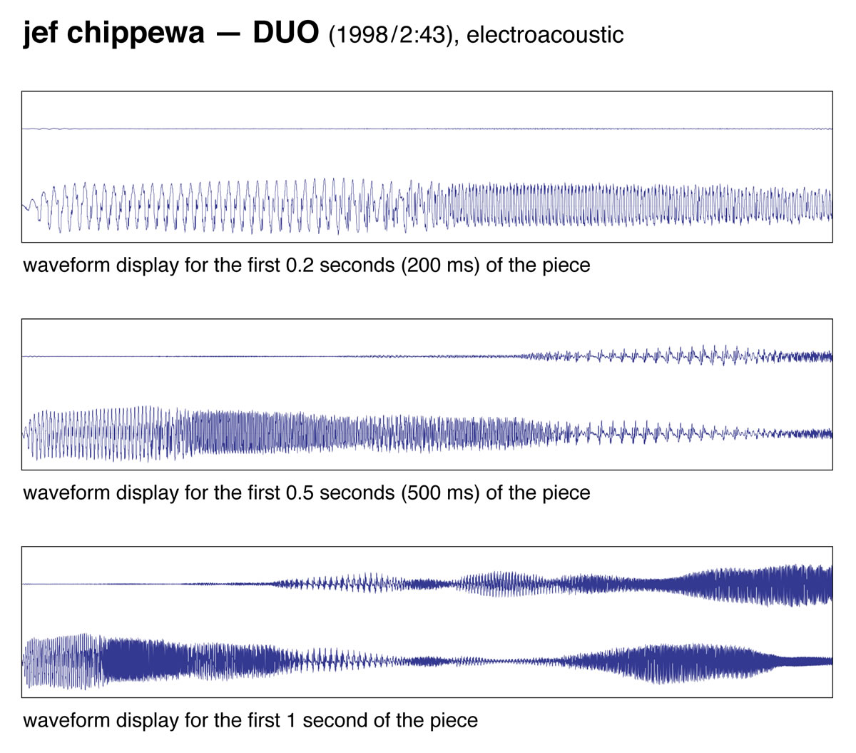
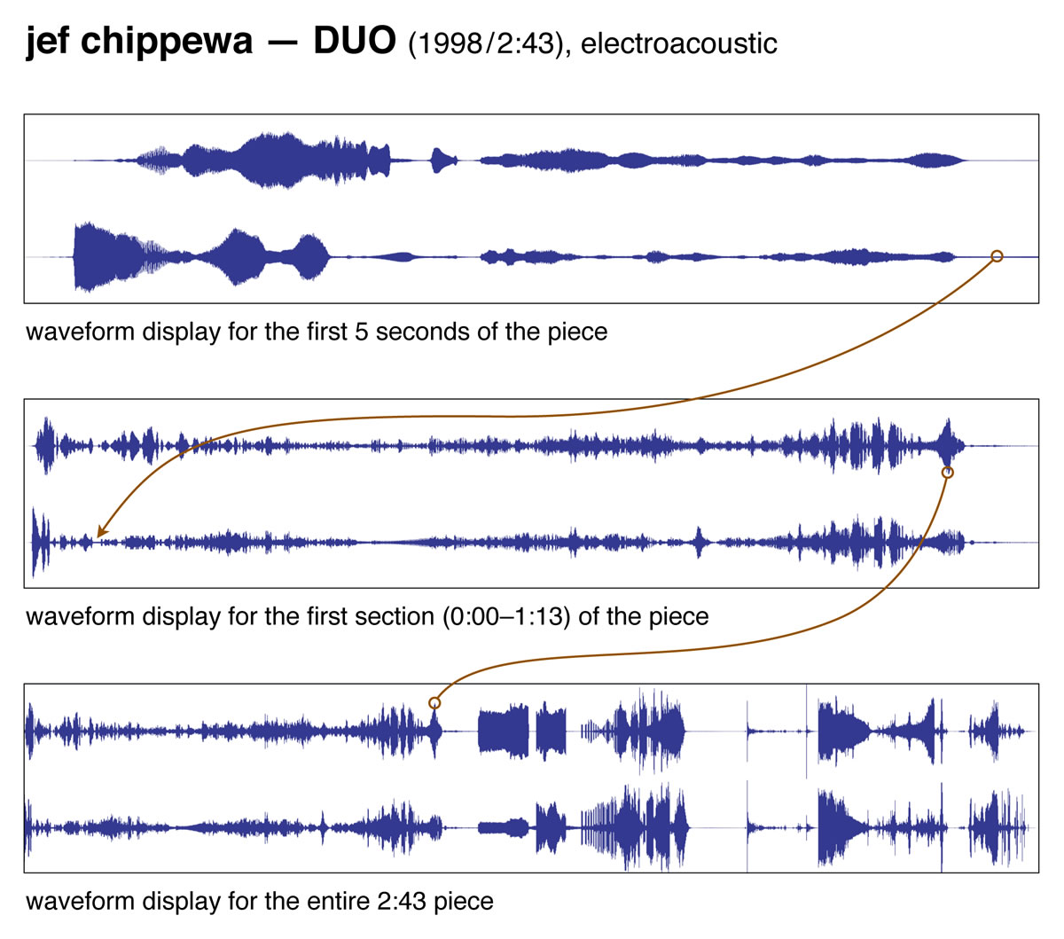
Time is represented horizontally and read left to right, while changes in amplitude are represented vertically as variations in the displacement of the waveform from the central horizontal line in positive (above) and negative (below) values. 1[1. Depending on the software and the user’s settings, the central line and outer boundaries of the waveform display may be represented as 0 (zero) and ±100%, 0 (zero) and ±1, -∞ (infinity) and 0 dB, or as 0 (zero) and x sample units.] With an extreme zoom, the shape of the wave itself is visible and shows in great detail the positive and negative variations in its amplitude (Fig. 1). When zooming out, the shape of the wave is temporally and graphically compressed and now appears as a solid mass, with variations in its thickness representing the contour of the combined positive and negative amplitude values of the waveform (Fig. 2).

What this form of notation lacks in artistry it makes up for, however, in functionality: this kind of representation of time and amplitude is certain to be familiar to virtually anyone who has worked with digital media in performance, in recording sessions or elsewhere. Even for those unfamiliar with it, this type of notation does not require any kind of specialized training — such as would be required to understand and follow traditional notation or spectrogrammes — to “get” the basic idea and to be able to follow the “score” as the sound file plays (Fig. 2, bottom; Audio 1).

Frequency Content

In the context of an art form that is intently concerned with complex timbres, one of the most outrageous inadequacies of waveform notation is the conspicuous absence of any representation of the frequency content of the sound file it represents. 2[2. It is possible today in some DAWs to show the frequency or spectral content in the form of, for example, a spectrogramme, alongside the waveform display — and in the same timeframe, if desired — but for the purposes of this discussion we consider the various types of visualization — notation — as separate entities.] The visualization of the variations in amplitude occurring in the sound file does not inform us if it contains a greater proportion of higher or lower frequencies, or rather a complex combination of a wide register of frequencies, not to mention how the frequency content changes over the course of the file or in the portion of the file visible on screen at a given moment (Audio 1; Fig. 2). Given two sound files with undifferentiated dynamic contours, it would be impossible to know that one contains, for example, noise-based percussive and gestural phrases and the other a performance of a piano sonata.

Loudness and Amplitude (not to be Confused with Dynamics)

Waveform display notation can be understood as a compressed, macro view of the actual form of the wave itself — the micro view, normally visible only when zooming in to such an extent that only one second or even less is visible on the screen (Fig. 1). This macro view offers an excellent way to represent very simple, monophonic sound. Because of the density of the actual waveform in normal viewing conditions (with anywhere from a portion of a second to the entire sound file visible on screen), the microscopic characteristics of the sound — the variations in amplitude occurring at the level of the microsecond — are neutralized, or rounded off (Fig. 2). 3[3. There is also the precision of the on-screen representation to take into account, which is directly related to the software settings and sample rate, and possibly screen pixelation. But this really doesn’t affect our understanding of the sound that is visualized.] However, as our aural perception also occurs at this macro level 4[4. For the sake of precision and focus, the question of psychoacoustics and perception will not be addressed here.], this is not, in itself, a problem for this particular form of representation.

Polyphony, or Layering

Nevertheless, already in the case of a mono (one-channel) sound file a more significant problem arises with waveform display notation, as it is a sum of all the parts (voices or layers, or individual components of a complex sound or sound mass) contained in the sound file. That is, the amplitude shown at a specific position in the waveform is a representation of the total amplitude (in negative or positive values) of all components present at that particular point in time. For this reason, the representation of the amplitude of even the simplest of waveforms is compromised with the introduction of a second component (or “voice”) in the same (mono) track — unless this new component has an identical dynamic shape as the first! Due to this phenomenon of amplitude summation, changes in amplitude that occur in individual elements within a single track are visible only in the most elementary dynamic situations — for example, where one sound remains rigidly at a constant level while another sound changes dynamically. However, a smoothly executed cross-fade between two components of a single (mono) channel may in fact appear graphically in waveform display notation as a seemingly unchanging level of amplitude.

Not to mention that, depending on the sonic content of the sound file, the actual acoustic levels may not at all reflect the perceived levels. In other words, scientific measurement of the intensity of a sound does not always compare to the experience of its perception by human ears. This is perhaps most easily explained by the fact that the waveform of an extremely loud but simple, high-frequency sound may in fact show a lower acoustic intensity than the waveform of a moderately loud but complex, very low-frequency sound.

Panning and Stereo Image

It is important to note that “panning” is to be understood not as sound that “moves” between two or more channels but rather as changes in amplitude of the contents of those channels that produce an illusion of movement to the listener’s ears. These changes may have either occurred “naturally” while recording the sound or source, or may be user-controlled facets of the piece. The problem of amplitude summation described above that is already present in the mono file quickly worsens in real working conditions, where stereo (2-channel) or multi-channel formats are the norm. Although the left and right channels of a stereo file can be shown as two separate waveforms such that the “weight” differences (amplitude) between them are evident (see esp. top of Fig. 2), this notation is — by itself 5[5. Today there are, of course, solutions to this problem, such as that discussed below in “Source Levels vs. Level of Source in a Mix,” but here we are focussing on inherent problems.] — as incapable of effectively displaying changes in the panning position of individual layers or voices as it is to showing polyphony within a single, monophonic track. Obviously, the situation deteriorates even more significantly when multi-channel (or multi-voiced) work is bounced to or combined in a stereo format and represented as waveform display notation.

Rhythm, Texture and Broader Temporal Aspects

Despite some of the inherent inadequacies in waveform display notation addressed above, this type of notation continues to be quite useful for the visualization of large-scale formal characteristics of a piece or recording. In the studio, the simplicity of this ubiquitous notation is extremely helpful for quick localization in sections of tracks or works. The ease with which it is possible in most contemporary DAWs to change vertical (representation of amplitude) and horizontal (representation of time) zoom factors of the waveform makes user navigation of this notation as efficient as possible.

But the inherently restricted amount of information it represents is problematic to varying degrees in many contexts. Imagine a collection of glitchy noise materials, all of a similar rhythmic character, that are combined to form a static texture in which these materials are periodically introduced or removed in such a manner that the overall density and amplitude remain the same for long stretches of time. In a waveform representation of such a passage, it may be impossible to recognize the precise points in time where specific changes occur, or where materials are introduced or removed. This is a similar problem as would be encountered in a piece with sustained sound at a constant dynamic that varies continuously in timbre. For example, in Barry Truax’s Riverrun (Video 1), the granular synthesis-generated sound is meant to be as continuous as a “river, always moving yet seemingly permanent” (webpage for Riverrun on Truax’s site, accessed 7 November 2017). Waveform notation is insufficient for such works because frequency is not represented at all and because the character of the rhythmic changes may be so simple, subtle or delicate that it is incapable of offering more than an unusable compromise between the timeframe and the rhythmic details or density of the materials that are visible on-screen at any given moment.

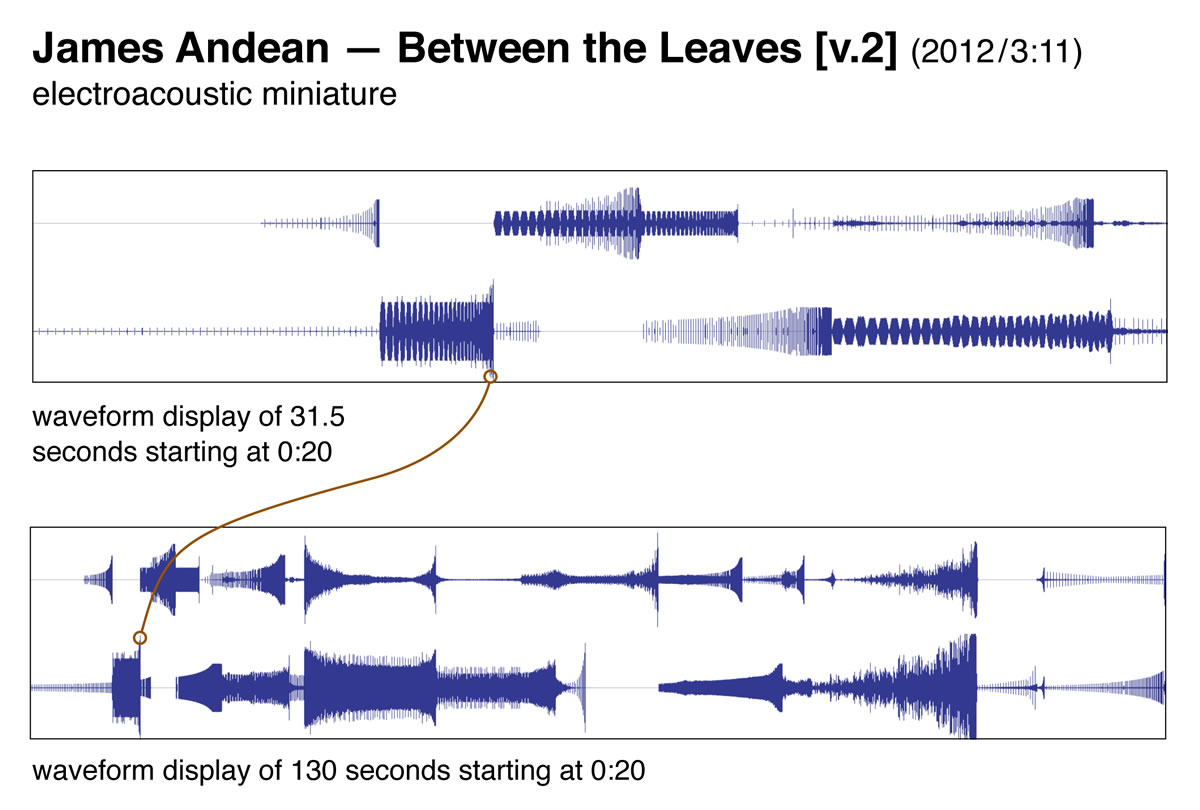
In a much sparser sonic texture comprised of discrete clicks, such as James Andean’s Between the Leaves (2012), this notation potentially offers a very effective non-metric representation of temporal positioning and changes in rhythmic density (Fig. 3). Although, when zooming out (i.e. adjusting the zoom factor so that more time is made visible in the same horizontal screen space), the graphic representation of the rhythmic changes could become so similar or dense that it becomes impossible to distinguish the individual rhythmic details. However, due to the extremely limited variety and density of materials encountered in Andean’s piece, the denser the notation (due to the zoom factor), the more effective it becomes in representing the “dynamic envelopes” of the individual tracks, or channels. Because of the abrupt nature of the clicking gestures’ onset and terminal points, the reductive palette of materials used and the fragmented, sparse texture, waveform display is quite likely the optimal choice of notation here 6[6. Although it could also be argued that even traditional notation could be used very effectively for this piece. With the individual voices shown on separate one-line staves and feathered beams indicating the speeding up and slowing down figures, traditional notation would be more effective in illustrating, at the very least, the polyphony composed into the work.]; the total lack of frequency representation would be largely unproblematic in this specific context.

Truly Proportional Notation

Despite its numerous inadequacies in the service of the graphic representation of complex sound, it should be noted that waveform display is one of the few types of notation that are truly proportional, where a specific length along a portion of the graphic is considered to be equal to a fixed and constant unit of time. In traditional, symbol-based notation through to the mid-twentieth century, a quarter note only extremely rarely occupies twice the horizontal space in the score as the symbol equal to half its value, the eighth note; the “empty” graphic space following these and other durational symbols is compressed in greatly varying proportion for reasons of legibility, performance praxis and norms of the music publishing industry. 7[7. The situation is significantly more complex than this statement would seem to suggest, but the topic of traditional, symbol-based notation can be discussed elsewhere at length.] This inherent compromise between visual representation and sounding duration does not challenge the reading or understanding of traditional notation — musicians see (or read, rather) beyond this incongruence… in specific contexts! However, absolutely proportional time-space notation is essential to any work for which a true representation of time flow is crucial to its understanding and/or performance.

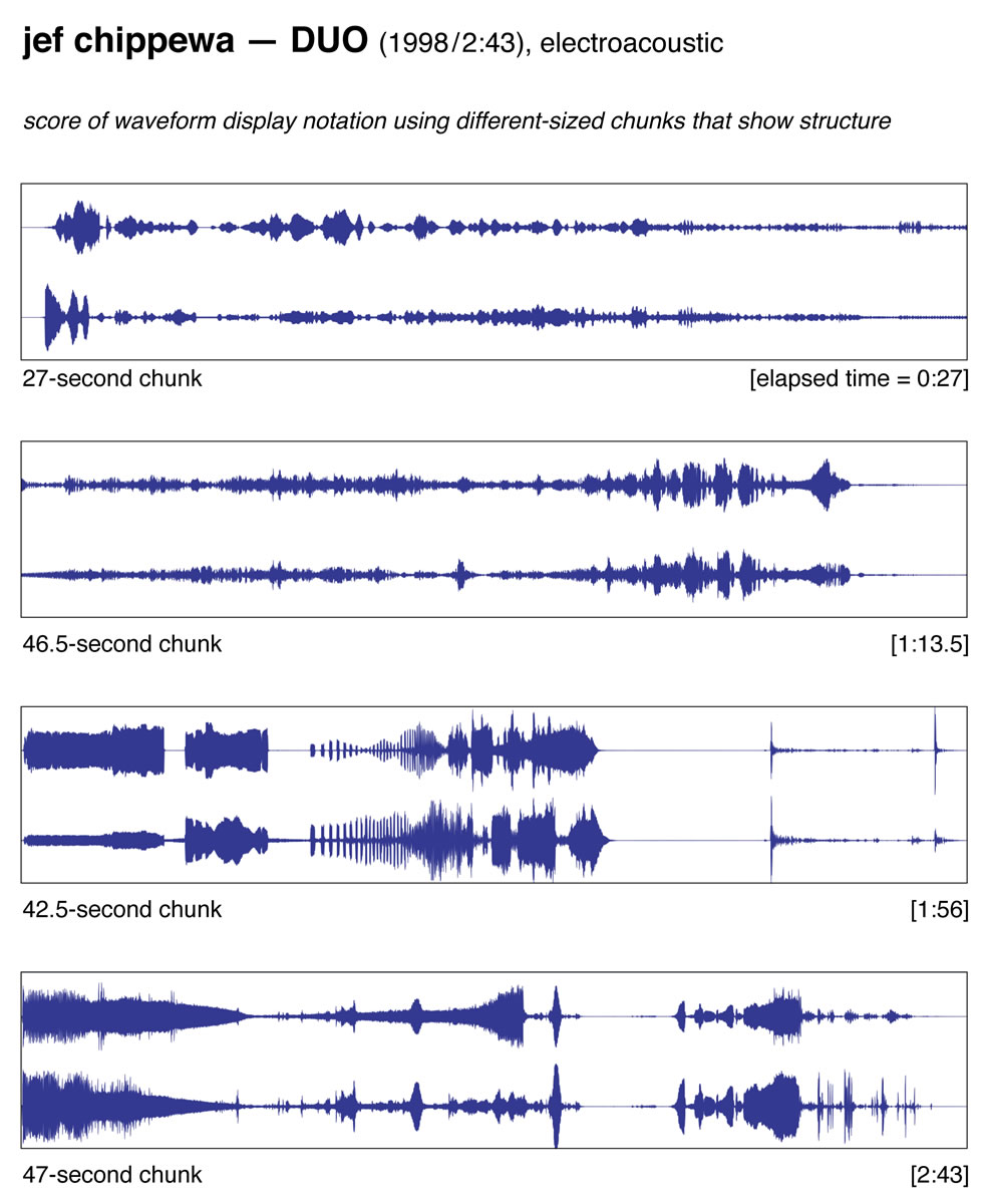
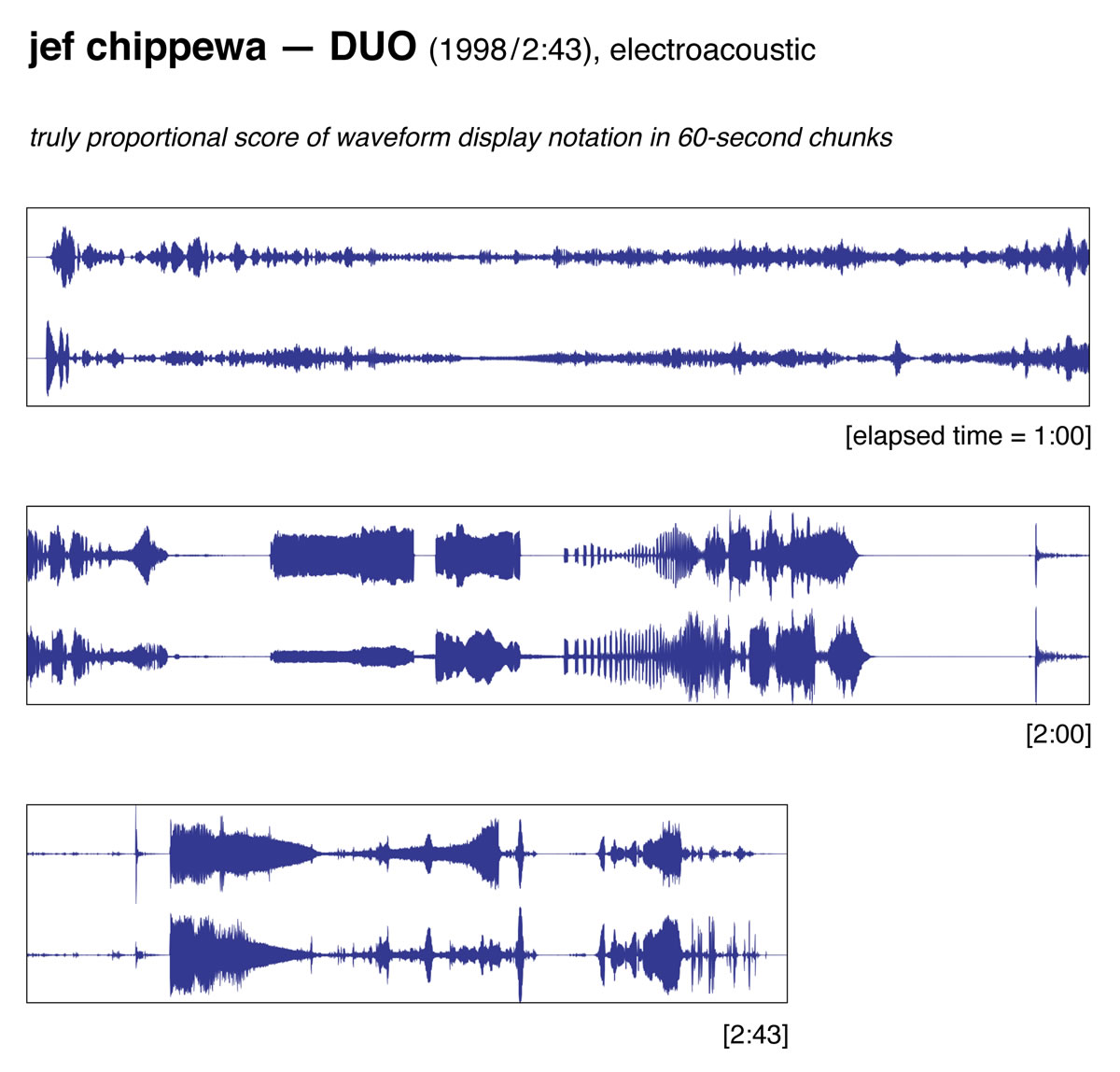
If the zoom level remains constant when taking all the waveform screenshots needed for the score, the spatial proportion is also constant throughout the entire score, i.e. across the entire collection of screenshots for the piece (Fig. 4). This is in stark contrast to traditional notation, which is built around symbolic rather than scientific representation. However, even in some contemporary circumstances of electroacoustic representation an insistence on absolutely proportional notation could prove to be impractical, or at the very least excessively and unnecessarily dogmatic. In order to properly represent some types of changes in sound or materials, and depending on the nature and density of the materials in different sections of the score, it could be useful or necessary to vary the time-space proportions — the amount of “real time” represented (made to fit) in a specific horizontal length in the score — between different sections of the piece. For example, a much simpler, sustained passage could be allotted a lesser amount of horizontal space than a passage that is rhythmically and dynamically more complex without any significant compromise being introduced into the score. Or slight difference in the length of portions of the piece could be made according to the structure and to avoid cutting in the middle of a musical or sonic gesture (Fig. 5). The important thing is that the durational proportions remain constant within or between individual chunks or sections of waveform notation where the visualization of these relations is important.

Zoom Level; or, Time Chunking

Contrary to traditional notation, no universal norms exist that are meant to regulate how much sound or music can or should be contained in one system, or in one horizontal chunk of waveform notation, or any other type of digital sound representation, for that matter. 8[8. The “norms” referred to here are perhaps not completely universal, but there are indeed many general guidelines that are followed by the majority of copyists and publishing houses and for all purposes and intents can be considered to be universal, albeit with perfectly justifiable exceptions. Again, another discussion for another time.] Some contexts may necessitate a broader perspective showing formal aspects of the work, while another may require the user to see its local characteristics in more detail. 9[9. This relates directly to the question of the role and function of the notation and/or score, a topic that will be touched upon in the final piece of this article series.]

The lack of detail in individual screenshots of longer time spans may make localization and navigating the sound file and score more difficult, whereas a very detailed zoom may become unmanageable because of the sheer excess of detail it contains, or for practical reasons such as the inordinate amount of page turns it might necessitate (if used, for example, as a printed score).

Some balance or even compromise will be needed to find the optimal macro-micro viewing percentage for a given context — no rules can possibly be set for this! The appropriate degree of detail needed and, therefore, the appropriate view percentage needed for the waveform notation, can only be judged on an individual basis, as the requirements of the notation may vary not only from one work to another but even between sections of the same work. From a general perspective, however, large-scale characteristics of the work can in many cases be represented very effectively using this form of notation.

Source Level vs. Level of Source in a Mix

Yet another problem arises with the use of waveform display notation that is directly related to its fundamental characteristic, the representation of variations in amplitude. When playing back an individual sound file, the apparent (psychoacoustic) intensity of its contents very often corresponds to its real (technically measurable) intensity, or, to put it more simply: what you see is more or less what you hear. 10[10. Psychoacoustics: yet another related topic that is too complex to address at length presently.] In real working situations, however, this may not necessarily be the case.

The waveform of a specific sound file perfectly reflects changes in amplitude (dynamic) found in the original recording but does not account for global or local variations in the level (“volume”) of that sound file within a mixing environment where any number of individual tracks, each with their own unique content and corresponding waveform, may appear in parallel. Indeed, in electroacoustic practices, it is hardly uncommon that sound materials that are both acoustically and perceptually “loud” in the original sound file are used at a severely decreased “volume” in the work into which they are integrated during the mixing stages.

There is no reason, however, that this discrepancy should trouble anyone, given the advanced affordances of today’s DAW user interfaces. So-called volume automation can be made visible in all or individual tracks so that both the source and mix levels of the sound file are shown throughout the portions visible on-screen. And in fact, the same possibility exists for panning, thereby helping resolve a related problem discussed earlier.

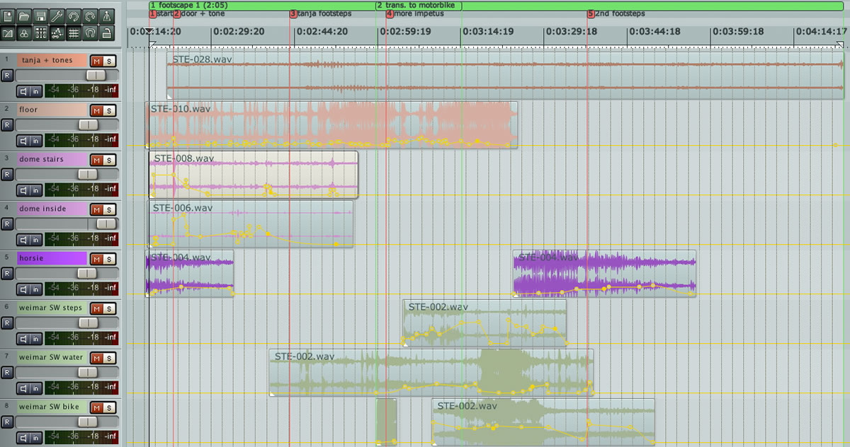
A screen capture taken while working on footscapes: one (2010/13) very effectively illustrates both the problem and solution (Fig. 6). The lowermost track in the image contains two clips excerpted from the same source recording, the first (starting at approximately 2:59 in the mixing environment) taken from a position in the second where the source levels are extremely high. But the mix level of the first clip is extremely low, this as-yet unrecognizable sound serving essentially to provide a little impetus to the more prominent gushing water sound that follows in the piece (in track 7); here, it is of very little consequence that one might possibly not be able to distinguish its identity. The mix levels of the second clip are generally higher than the first and are varied not to manipulate the timbre and perception of the sound (as was the case for the first), but rather to reinforce its inherent dynamic contour — that of a motorbike arriving from a distance, passing close by the mic and continuing off into the distance — as well as to boldly reveal its identity and control its presence within this slightly more complex mix.

The visualization of the volume automation makes it possible to see relations between the source and mix levels of the two clips, as well as between these and other clips used in the piece, and to help analyze and understand to some extent the different approaches to their use that would otherwise not be possible with waveform display notation.

Conclusion

Notation is a means to represent sound in a visual form, whether that which is notated is intended for live performance or as an analytical tool. In electroacoustic practices, a variety of traditional and domain-specific approaches (e.g. waveform display, spectrogramme) to notation are encountered in varying proportion. Each of these will be addressed individually in detail in subsequent texts. It is hoped that the breadth of this lead-in discussion of waveform display notation provides a solid basis from which it will be possible to better comprehend the impact of individual aspects of the various forms of notation, as well as to judge their effectiveness in representing or servicing the diverse musical and sonic circumstances encountered in the wider realm of electroacoustic practice.