A Generalized Introduction to Modular Analogue Synthesis Concepts
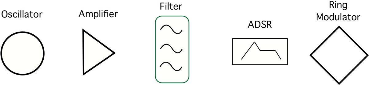
The key concepts behind modular analogue synthesis provide a foundation for an understanding of a very wide range of synthesis techniques available today. This article assumes some familiarity with most basic modular modules such as an oscillator, amplifier, filter, ADSR, ring modulator, etc. Most definitions and references can be found in Wikipedia.
There are essentially three kinds of synthesizers: analogue, digital and hybrid (analogue with digital features). One of the main differences between the “pure” analogue and the other types is that the “pure” analogue does not have digital components or “memory”, except in larger compound modules, such as the step sequencer. This article does not deal significantly with digital components, i.e. modules dependent upon memory functions, such as the digital delay, digital reverb etc., although such modules are increasingly to be found in modular synthesizers.
Definitions and Basics
The modular analogue synthesizer is an electronic instrument. YouTube has many tutorials on an enormous range of applications and they run from the high school student who is showing his equipment, to well-considered and prepared explanations. One of the major differences between them is their degree of accuracy and, notably, precision in their use of terms. To help, this article uses the following specific definitions.
Sound. An acoustic wave, characterized by variations in pressure — the amplitude of the wave.
Signal. An electronic wave, characterized by variations in voltage — the amplitude of the wave.
It follows that there are no “sounds” in the synthesizer, only signals. Signals will be described in terms of their functions, that is, how they are used or what they do.
Potentiometer. The device behind the knobs, most frequently used to change amplitude, frequency or spectrum (Fig. 1).
Register. The description of which (frequency) area a sound occurs in. For example, the piccolo is in the high register, the bass drum is a low-register instrument.
Range (bandwidth). A term of some confusion as it is often used to mean two or more different things — one of which is “register”. Range is synonymous with bandwidth in that it tells about the upper and lower limits of a condition, for example, an average singer has a range of about a major tenth, or a standard VCO has a range of 10 to 15 octaves. Range is often used to describe the register, as in mid-range EQ, thus the confusion.
Audio. The frequency range of around 25 Hz to 15 kHz
Subaudio. The frequency range from 0 Hz to around 25 Hz
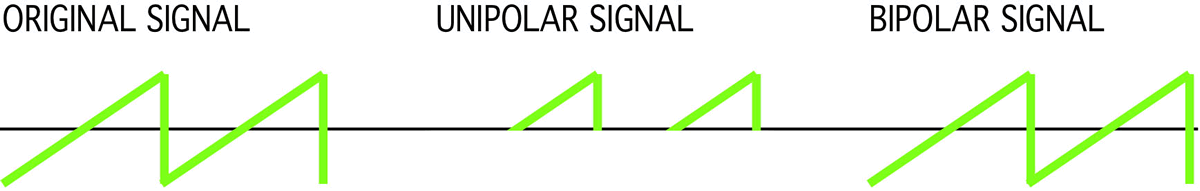
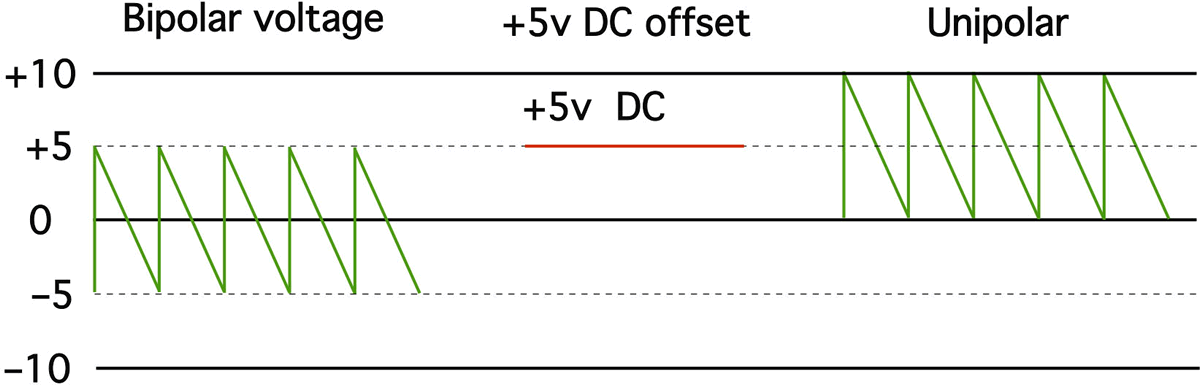
Unipolar. The signal can only have positive (or only negative) values (Fig. 2, centre).
Bipolar. The signal can have positive and negative values (Fig. 2, right).
Distortion. Unwanted alteration of a signal.
Analogue. Continuously variable.
Stepped. Discrete.
Continuous. The output signal is always present.
Transient. The output signal is only present when the module is triggered, e.g., ADSR.
Oscillator. A continuous source of periodic waves.
Noise. A continuous source of an aperiodic wave.
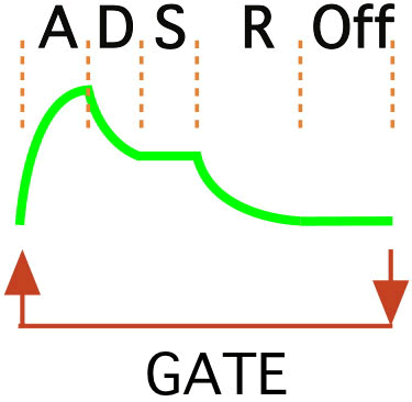
ADSR. A transient voltage source.
Amplifier. A voltage multiplier.
Filter. A frequency-dependent amplifier.
Parameter. A characteristic, or an element, of a module. Examples of parameters include:
- Oscillator — frequency, pulse-width, wave shape;
- Amplifier — amplitude;
- Filter — cut-off frequency, resonance (q), bandwidth, slope;
- ADSR — attack time, decay time, sustain level, release time.
Voltage control. The control of a parameter of a module by a voltage. The response is proportional to the control.
Graphics
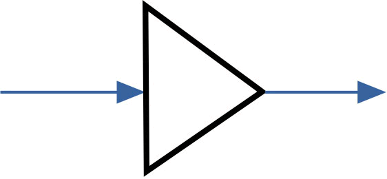
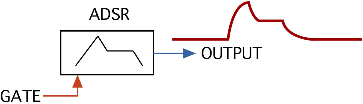
Block diagramme. Shows the relationships of modules in an abstracted graphic form (Fig. 3).
Some modules will be given a specific shape, such as an oscillator, an amplifier, a filter, an ADSR, ring modulator, etc. Only some shapes are standardized.
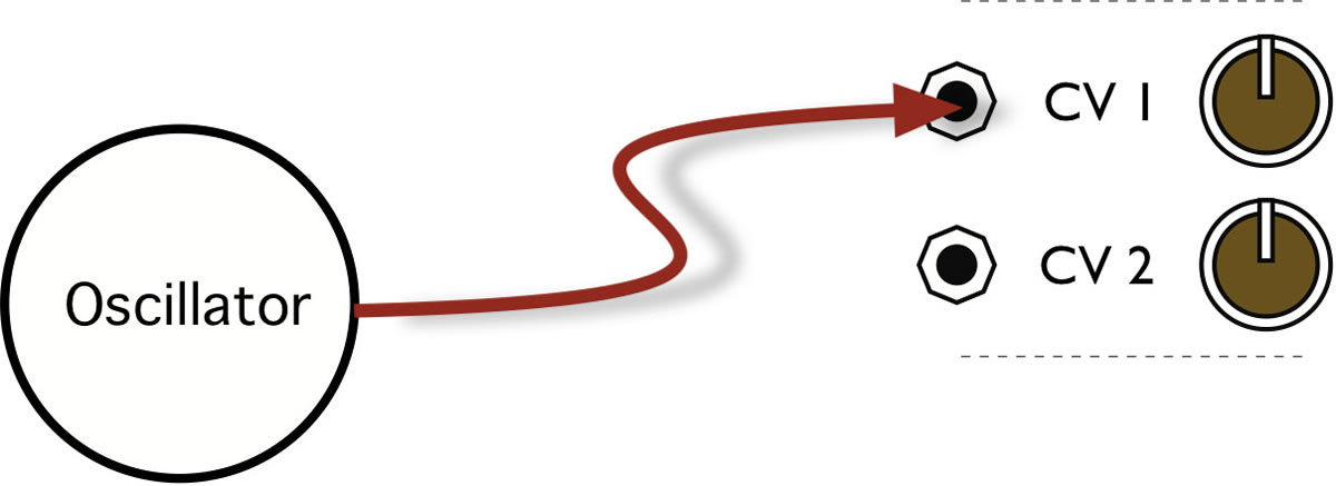
Patching diagramme. Shows how to connect modules together on a specific instrument. The patching diagramme (a patch) in Figure 5 is similar to the block diagramme shown in Figure 2, with a control voltage added to the source oscillator.
Module Types
Modules types fall into three categories: source, processor and compound.
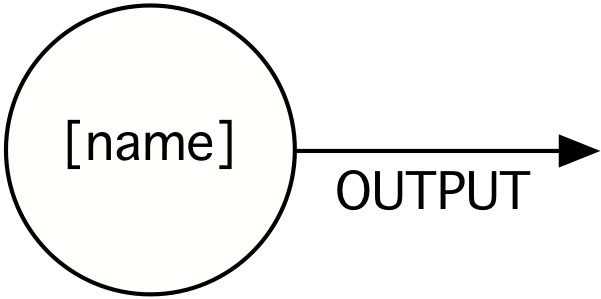
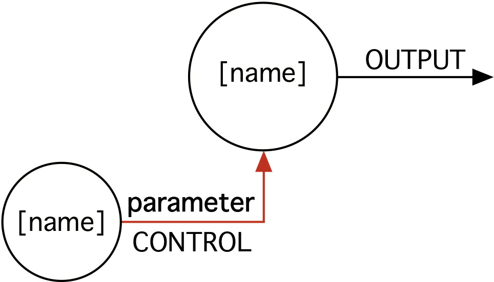
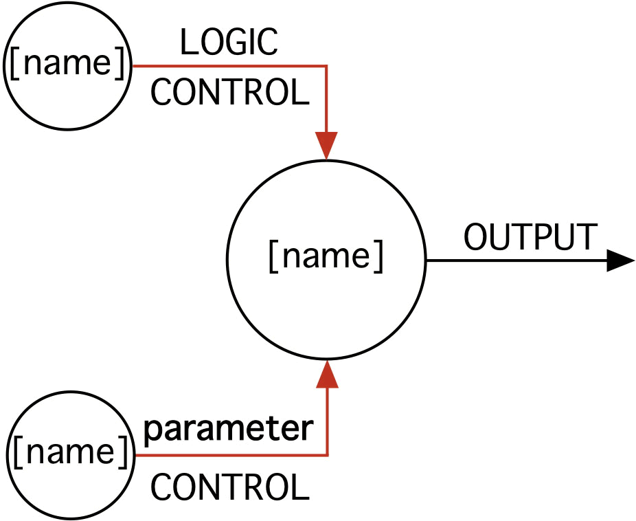
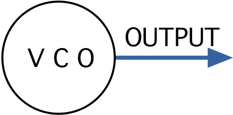
Source module. Has one (or more) outputs, e.g., noise. It has no (signal) input (Fig. 6), may have (one or more) parameter control inputs (Fig. 7) or may have logic inputs (Fig. 8).
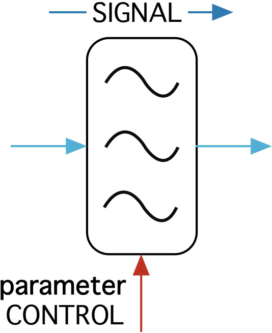
Processor module. Has a signal input and a signal output (Fig. 9), e.g., a filter. The signal may be an audio signal or a control signal; it may have (one or more) parameter control inputs (Fig. 10) or may have logic inputs (Fig. 11).
(Note that unusually, the logic input in the block diagramme may be shown above or below the module.)
Compound module. A combination of several basic modules into one module, for example an envelope follower, a step sequencer or a vocoder.
Source Types
Continuous source. Examples of continuous sources include oscillators (periodic waveshape), DC source (fixed, invariant voltage) and noise sources (random / aperiodic waveshape). Noise source modules with various colour outputs are compound modules, for example noise followed by a filter.
A DC offset source allows for the reference level of a signal to be modified by the addition of an offset voltage through a control input. This is useful when, for example, working with unipolar VCAs, which only respond to positive control voltages (Fig. 13).
Transient source. Examples of transient sources include the ADSR, keyboard, strip controller, etc.
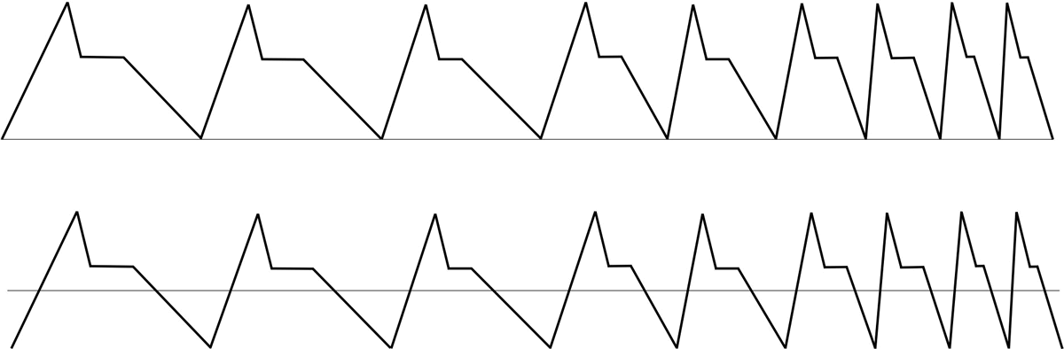
A line-segment generator is a source that when triggered, produces a series of rising, falling or sustained voltages, the most common being the AR (attack-release), ASR (attack-sustain-release), ADR (attack-decay-release) and the most frequently found, ADSR.
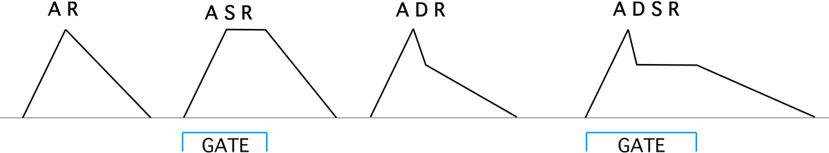
A trigger is necessary to initiate the cycle; the sustain requires an external gate. The A, D, S and R could all be voltage controlled. The ADSR is a member of a family of line-segment generators, which may be made continuous with the addition of an “off” time (Fig. 16). At the end of the “off” time, a trigger/gate is sent to the (logic) control input. This method would produce a continuous output.
With very short times on the stages, the module could be used as a variable waveshape oscillator.
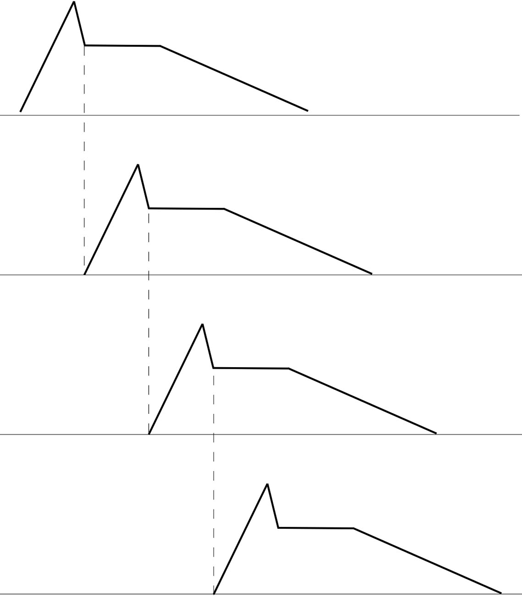
There are compound versions of this module that output a trigger with every change of stage. This can allow for sophisticated automated sound projection. In Figure 18, at the end of the decay phase, a trigger/gate fires the next ADSR.
External source. Audio source (microphone or line input) as a source of any arbitrary wave shape (signal).
Processor Module Types
Spectrum Modules
Filters. Low-pass, high-pass, band-pass, notch (band stop or band reject), all-pass, VCF (voltage controlled filter).
Equalizers. Graphic equalizers, parametric equalizers.
Spectrum modifiers. Phase, flange, chorus.
Wave shapers. Dividers, octavers, distortion.
Amplitude Modules
Amplifiers. Attenuators, unity gain amplifier, preamplifier, mixer, inverter, panner.
Multipliers. VCA (voltage-controlled amplifier, a two-quadrant multiplier), ring modulator (four-quadrant multiplier).
Time Modules
Reverb. Spring reverb.
Echo/Delay. Delay line.
Miscellaneous Modules: Routing
Switches. Unidirectional switch, bidirectional switch.
Counter. Counter.
Compound Modules
Compound modules vary in size and complexity from an envelope, to an envelope follower, to a vocoder or a multi-step sequencer.
Function Type
All signals in the instrument are the same in terms of being electricity. The difference between a(n audio) signal path, a control and a logic / timing signal is how the signal is used — its function.
(Audio) Signal path. The (audio) signal path is part of the path to an audio output.
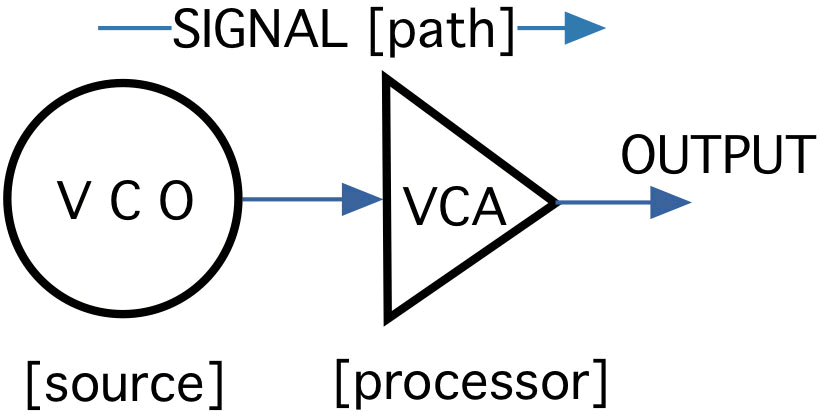
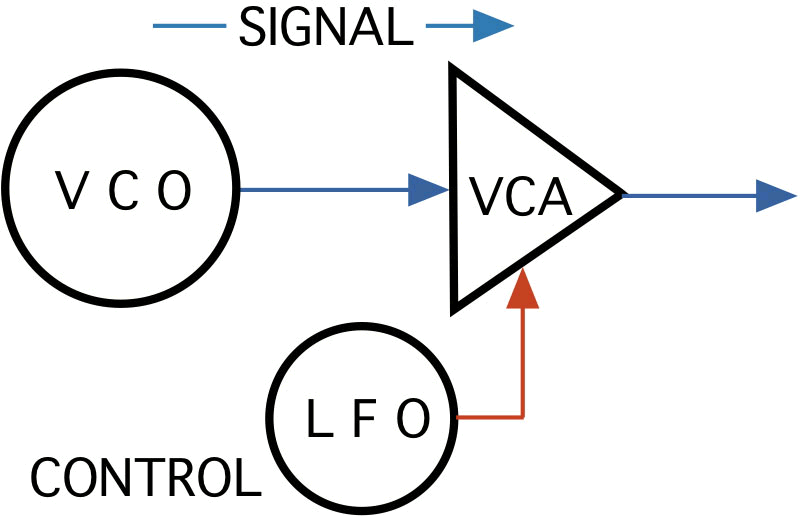
In Figure 19, the (audio) signal is output from the VCO, goes into the VCA, and the output from the VCA goes to an output channel. Note that the normal direction of the (audio) signal is indicated in the block diagramme moving from left to right.
Control. The control signal is used to control a parameter on a module. It may be stepped or continuous.
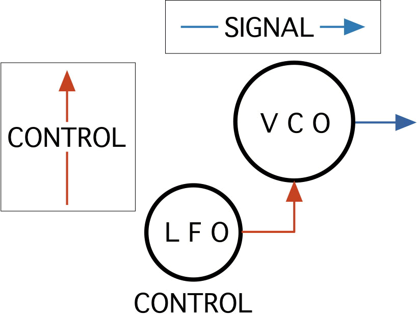
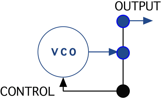
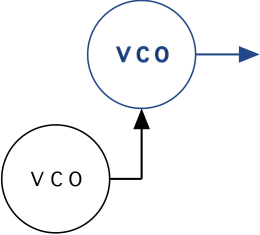
In Figure 20, the (audio) signal is output from the VCO. The frequency of the VCO is being controlled by an LFO. The output signal from the LFO is functioning as a control voltage. Note that (parametric) control voltage normally enters the controlled module from below. The normal direction of the control voltage is vertical.
Logic / trigger. The signal is used to change the state of a module, or trigger an action.
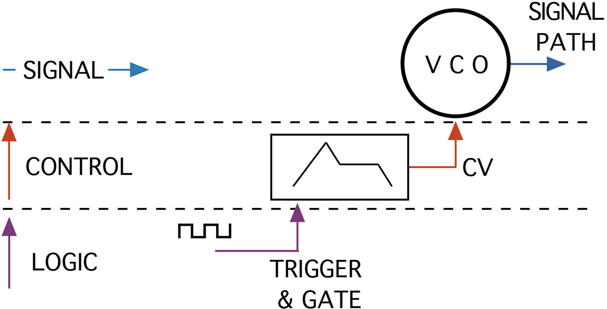
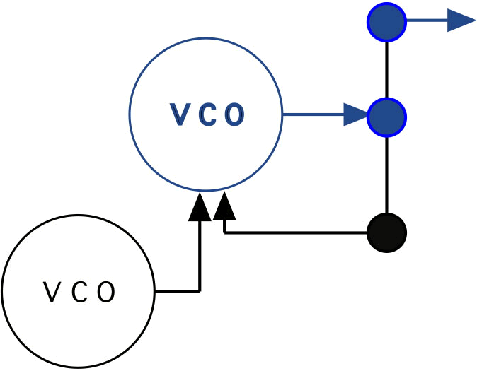
In a block diagramme, the logic signal usually enters the controlled module from the bottom, however entry from the top is used in some circumstances. Figure 21 shows three “levels” in the patch — the output of the VCO is part of the (audio) signal path. The frequency of the VCO is controlled by an ADSR, the control voltage (CV). The ADSR is a transient source and only fires when a trigger and gate (logic function) are present.
Examples and Applications
An Invented Block Diagramme Explained
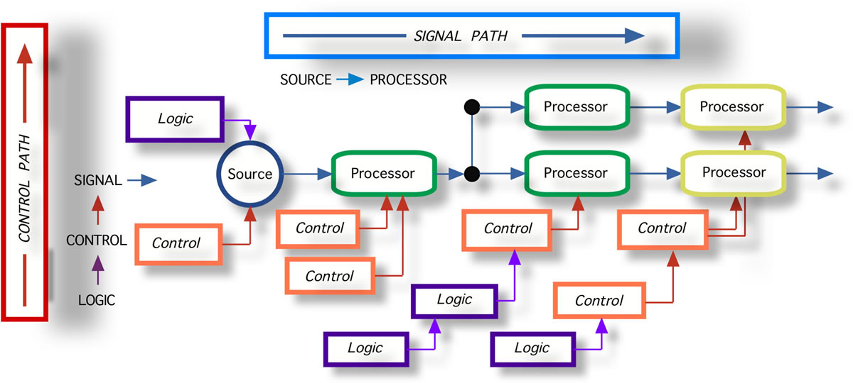
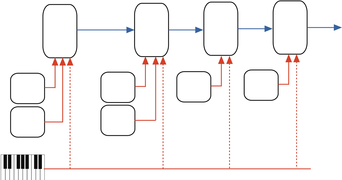
An invented block diagramme showing all of the types of paths can be used as a general guide to understanding the terms defined above. Note that (audio) signal paths usually run left to right, (parametric) controls usually run up into the bottom of the symbol and logic / trigger paths enter from above or below (Fig. 22).
Starting from the left of the diagramme in Figure 23, the (audio) signal path has one source and five processors:
- The source has one parametric control and one logic control;
- Processor 1 has two separate parametric controls and its output is split;
- Processor 2 has no controls;
- Processor 3 has one control;
- Processor 4 has one control, triggered by a logic module;
- Processor 5 has one control — the same control as Processor 3.
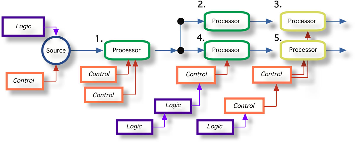
There are a total of five control paths in the diagramme, some of which have multiple layers. For example, control paths 4 and 5 each have three layers of controls.
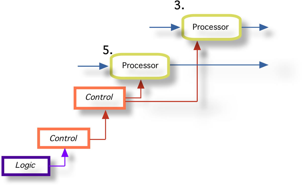
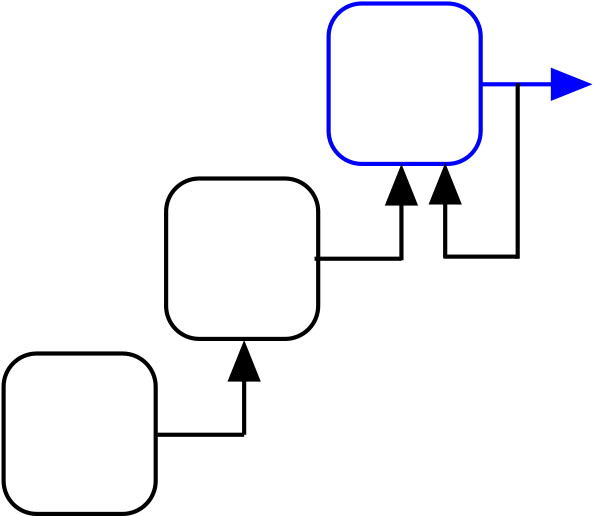
Another way to draw the processors 3 and 5 from Figure 23, so as to avoid the control output going underneath processor 5, is to move processor 3 to the right so that the patching path is clearer (Fig. 24).
Voltage Control of Module Parameters
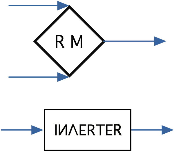
Not all modules have parameters that can be controlled. Examples include the ring modulator, a processor with two inputs and one output, and the inverter, a processor with one input and one output (Fig. 25). Sometimes an inverter will have a DC offset knob, and this forms a type of compound module: inverter and DC offset.
The basic oscillator has one parameter that can be controlled: the frequency. The frequency of the oscillator will vary with the voltage applied to the control input. Figure 26 shows a voltage-controlled oscillator (a) whose frequency may be changed by turning a built in knob (b) or by applying a control voltage to a control voltage input (c).
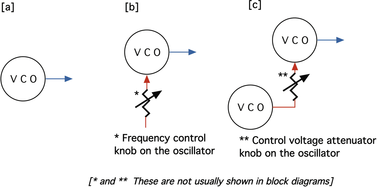
There is an attenuator on the control voltage input (Fig. 27, right), but this is not usually shown in the block diagramme.
Amplifiers
The voltage-controlled amplifier (VCA) is an often misunderstood module because, in common usage, to “amplify” means to “increase the signal level”.
Most modular systems have two kinds of amplifiers on them: VCA and preamplifier. The standard VCA is a unity gain amplifier — the maximum gain is x1, so that the output level is never higher than the input level. It could be considered that this module is a “voltage-controlled attenuator”.
The preamplifier module will have a maximum gain greater than x1. This is needed to bring certain external signals into the voltage range for most efficient use of the modules. A microphone or guitar may need a gain of x1000 or more. Preamplifiers are not usually voltage-controlled.
A preamplifier can be used as a wave-shaper such that the gain may be of a high enough level that input signals are clipped.
As defined above, an amplifier is a voltage multiplier. That is:
input voltage x multiplier = output voltage
| Input voltage |
Multiplier (CV) |
Output voltage |
| 1 V | 1 (unity gain) |
1 |
| 1 V | 0.5 | 0.5 V |
| 1 V | 0.2 | 0.2 V |
| 1 V | 0 | 0.0 V |
| 1 V | -2 | 0.0 V |
| 1 V | 5 (*) | 5.0 V |
*) This is not possible with a standard VCA, only with a preamplifier module.
There are three things to note in the table above:
- An amplifier can output a lower voltage than is at the input — this is attenuation.
- Being unipolar, if the multiplier — the control voltage — is less than “0” (a negative number), there is no output, as the VCA control voltage input is unipolar.
- The maximum output level of the standard VCA is not higher than the input level.
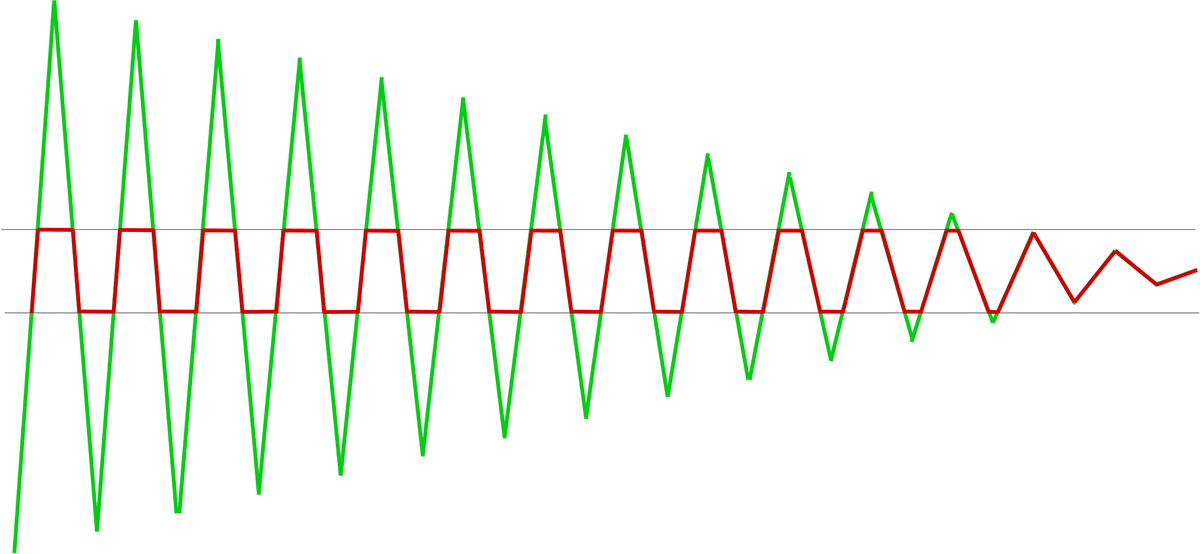
In Figure 28, the decaying triangle wave (in green) is amplified beyond the limits of the amplifier. This leads to clipping, flattening the top and bottom of the wave (in red). As the triangle wave diminishes in level, the wave changes shape from a quasi-square wave to a clipped triangle wave and eventually to a triangle wave. This change of wave shape is a change in the number and intensity of the partials. It sounds somewhat like a low-pass filter closing.
The technique of clipping a signal can be useful to waveshape a transient attack onto a signal, as the transient portion of the wave will be clipped by the amplifier limits, but the sustained portion will not be clipped. This cannot be done with a standard VCA as this requires the amplifier gain to be greater than “1”.
Filters and Equalizers
The filter, a processor, can be understood as a frequency-dependent amplifier.
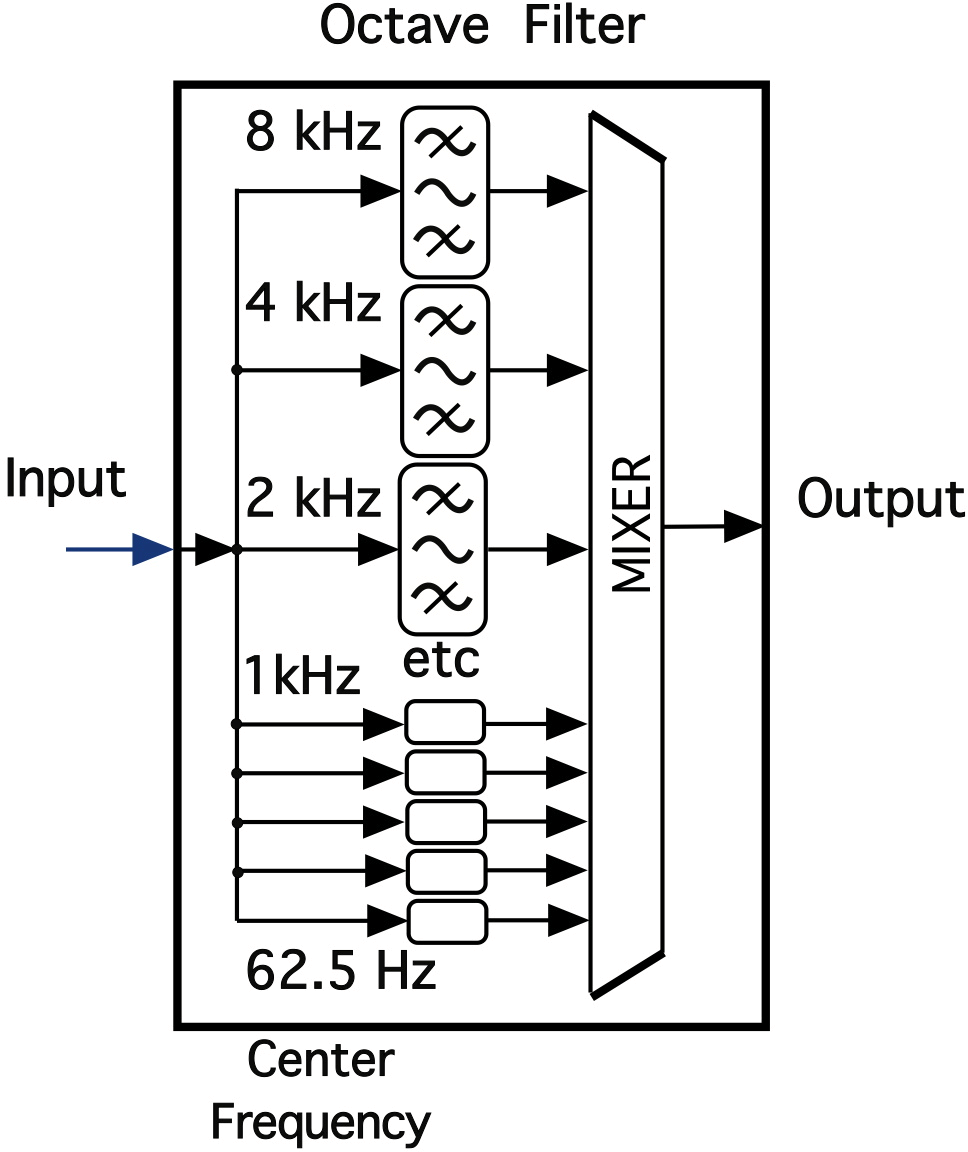
The structure of the octave EQ shown in Figure 29 reflects its compound structure, with eight bandpass filters and a mixer. The controls have been omitted for clarity. This multiband design is at the heart of the analysis section of a vocoder.
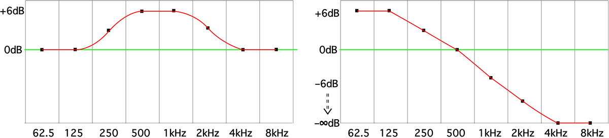
A stylized frequency response of an octave equalizer (Fig. 30) shows a 6 dB frequency boost from about 350 Hz to 1.4 kHz (on the left) and a 6 dB bass boost followed by a low-pass filter slope starting at around 125 Hz (on the right).
It is noteworthy that the equalizer has boost available, which allows it to become a frequency- and amplitude-dependent waveshaping / clipping module.
There are multiband equalizers where the output of each filter is available independently. Other designs include control of centre frequency and bandwidth (q) of each filter. With a 10-band filter, there could be more than 40 controls, including, for each band: input level, centre frequency, cut/boost, q and output level. Each of these could be voltage-controlled, giving the module some 50 knobs and 50 sockets. With this number of controls of the parameters, they are often called parametric equalizers.
Oscillator
The basic oscillator is a source of periodic voltage change. In most oscillators this is followed by a waveshaping circuit to produce a variety of waveshapes. The outputs of the waveshaper may be mixed together to produce intermediate shapes. Pulse-width modulation (PWM) is a specific form of wave shaping, usually voltage-controllable.
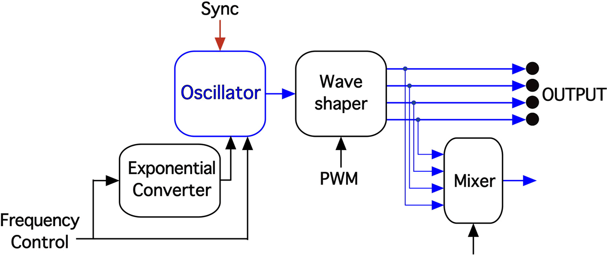
The response to control voltages of most oscillators is exponential, with a change of one volt at the control input changing the frequency of the oscillator by one octave, thus, one volt per octave (1V/oct). This uses an internal module — an exponential converter — as VCOs are by nature frequency linear, one volt producing the change of a fixed range, e.g., one volt per 500 Hz. The “classic” FM sound as found for example on Yamaha’s DX-7 is (frequency) linear modulation.
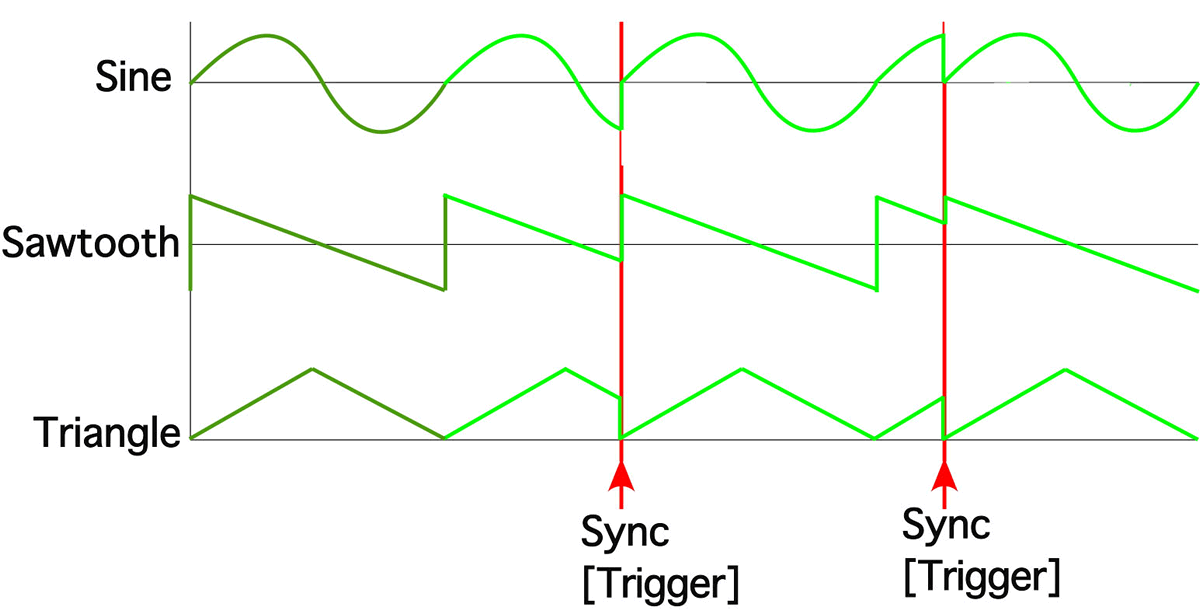
VCOs may also have a logic input that resets the oscillator to a 0° phase position, the sync input. The sync input responds to a trigger (Fig. 32).
Noise and Random
Noise and random voltages can find many uses in patches as ways of introducing a very slight to great degree of unpredictability, or fuzziness to signals. The noise or random voltages cause variations in frequency when applied to a VCO (Fig. 33), or can be used, for example, to cause variations in the amplitude (Fig. 34, left) or centre frequency of the filter (Fig. 34, right).
The Simple Switch
A switch is a logic-controlled device that changes state with the application of a trigger. In the example at the left in Figure 35, the trigger selects first one input, then the other input. In the example on the right, the switch is used to route an input to either of two outputs.
The Logic of Triggers and Gates
A trigger (usually) is a fast-rising edge that when applied to a trigger input, initiates an action. The trigger can be continuous in action, such as the rising edge of a pulse / rectangular wave from an oscillator, often used as a clock. A trigger can also be transient, such as the output from occasionally pressing a button or a key.
A gate is a signal above a certain level — a threshold — that “allows” an action to take place. It is most frequently found represented by a pulse / rectangular wave, with the levels being a logical “0” (low), or “1” (high).
Many modules combine the functions of the trigger and the gate and call them a “gate”. The trigger is sometimes called a “retrigger”. The terminology can be confusing, but simplified by the following diagrammes.
The ADSR, Trigger and Gate
One of the first commercial ADSRs was manufactured by MOOG. To trigger the ADSR, it was necessary to have a trigger and a gate. The module used two different kinds of plugs and sockets for the two functions.
When a gate was present — an “and” condition — a trigger would initiate the ADSR cycle.
Figure 36 shows the output of an ADSR, in relation to triggers and gates.
| Position number |
Trigger | Gate | Output |
| 1 | √ | nil | |
| 2 | √ | √ | initiates ADSR cycle |
| 3 | falls | initiates “release” phase | |
| 4 | √ | nil | |
| 5 | √ | √ | initiates ADSR cycle |
| 6 | √ | √ | reinitiates “attack” phase |
| 7 | √ | √ | reinitiates “attack” phase |
| 8 | √ | √ | reinitiates “attack” phase |
| 9 | falls | initiates “release” phase |
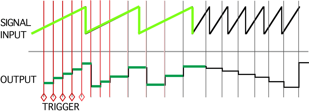
The Sample and Hold, Track and Hold
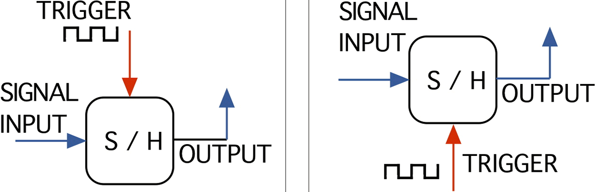
The sample and hold is a voltage quantizer, with a signal input and a trigger input (Fig. 37). Whenever a trigger — a rising edge — is presented at the trigger input, the instantaneous input voltage is sampled, this value is held and is available at the output.
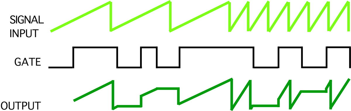
The track and hold has a signal input and a gate input (Fig. 38). Whenever a gate is present at the gate input, the input signal is passed through to the output. When the gate goes low — back to “0” — the voltage is sampled and that value is available at the output.
The Comparator
The comparator is a logic device that compares two values and outputs based upon the design of the module. This is an introduction to the concept and basic types. These modules are often included in larger compound modules.
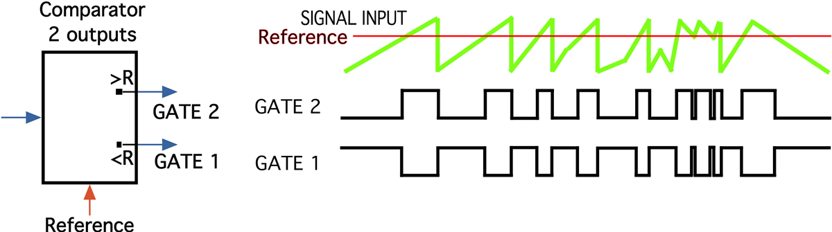
The 2-output comparator has a signal input, a reference level (which may also be a logic input) and two gate outputs (Fig. 39). When the signal level is below the reference level, a gate (high) is present at output (gate) 1. When the signal level is above the reference level, a gate is present at output 2.
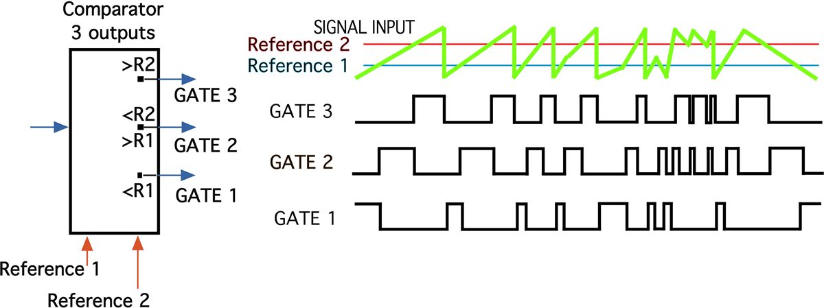
The 3-output comparator has two reference levels and outputs gates accordingly at output 1, output 2 or output 3 dependent upon the input signal level and the reference levels (Fig. 40). Notice that this “simple” module is able to produce streams of gates of considerable complexity regarding attack times and durations.
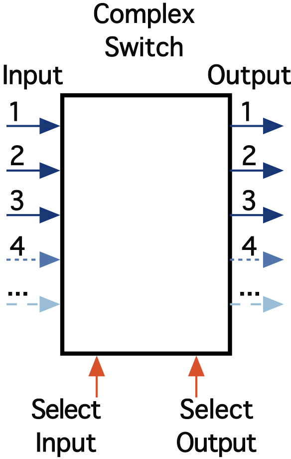
The Complex Switch
Switches are useful “routing” devices, being able to select from a number of inputs and directing to a number of outputs. The simple switch described above uses a trigger to switch states. A more sophisticated module could select from any number of inputs and direct to any number of outputs (Fig. 41). These are compound modules, often titled Voltage-Controlled Switch or Sequential Switch.
Envelope Follower
Depending upon the design, this module could have as few as one input and one output, or up to four inputs, up to five outputs and three or more control knobs. In the example shown in Figure 42, there is one signal input, one control input and two outputs: a signal and a gate. However, note that there are four separate functions (modules) inside this module: an amplifier, a half-wave rectifier, a low-pass filter and a threshold detector.
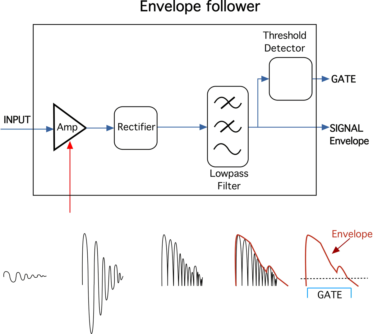
The signal whose envelope is to be followed (Fig. 42) appears at the input and is amplified. There may be an external gain control. This amplified signal is half-wave rectified so that it is a unipolar signal rather than bipolar. This signal is processed by a low-pass filter, usually with a cut-off frequency below 30 Hz, which smooths out the wave, producing the “envelope signal”. A threshold detector outputs a gate. Below the block diagramme is an example of the stages of transformation of the wave.
Vocoder
The vocoder has two stages: analysis and synthesis (Fig. 43). In the analysis stage, the incoming signal is bandpass filtered into 8–15 bands, more or less. The output of each filter is processed by an envelope follower, producing ±8–15 transient voltages.
The synthesis stage has a signal input, which is passed through the same number of bandpass filters, followed by an amplifier. In some designs of the vocoder, the transient voltages of the analysis stage are directly connected to the control inputs of the amplifiers of the synthesis stage. The outputs of these amplifiers are summed, and the “spectral outline” of the analyzed signal has been applied to the signal in the synthesis stage.
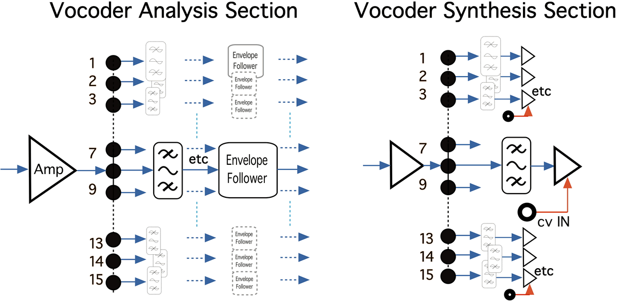
Another design allows for the “cross-patching” of the generated transient voltages so that the relationship between the analysis and synthesis bands is arbitrary. For example, the transient voltage of the 500 Hz band, could be applied to the amplifier on the 2 kHz synthesizer stage. This allows for the exchange of frequency band profiles.
Multiple Levels of Control(s)
Much of the flexibility and nature of continuous change in modular systems comes from being able to have many “layers” or levels of controls — both parametric and logic.
Self-control is one of the potentially very interesting control levels. It relies upon the creation of a feedback path (Fig. 44). Depending upon the module involved, such as a filter on the verge of oscillation, the system can become unstable, producing unpredictable results.
The most commonly found control is one module modulating another (Fig. 45).
This can be expanded with the addition of self-control (Fig. 46).
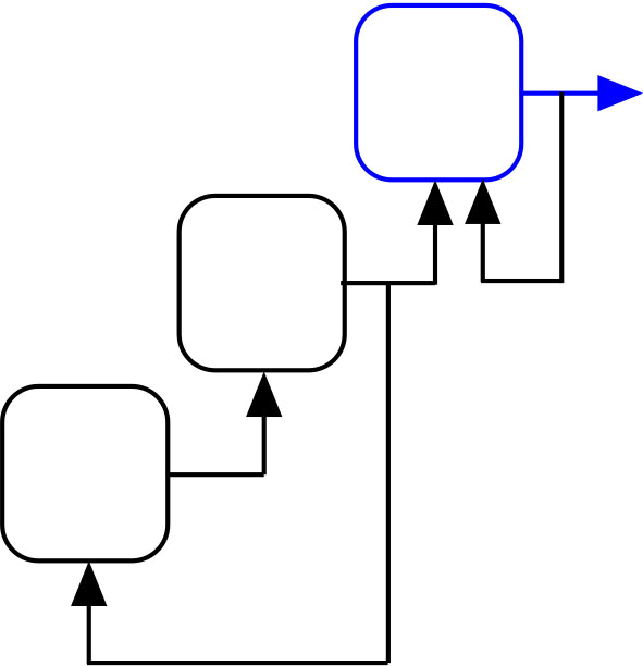
Multiple levels of controls can be set up so that, for example, one modulator can modulate another modulator (Fig. 47).
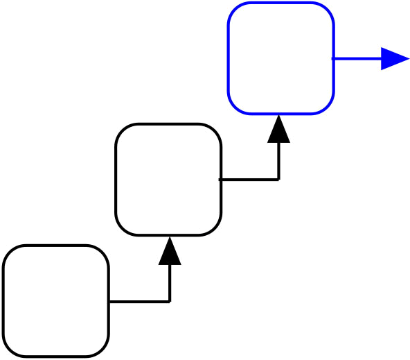
Figure 48 shows the same as Figure 47, but with a little self-control.
And in Figure 49 there is self-control in a feedback patch between levels 2 and 3.
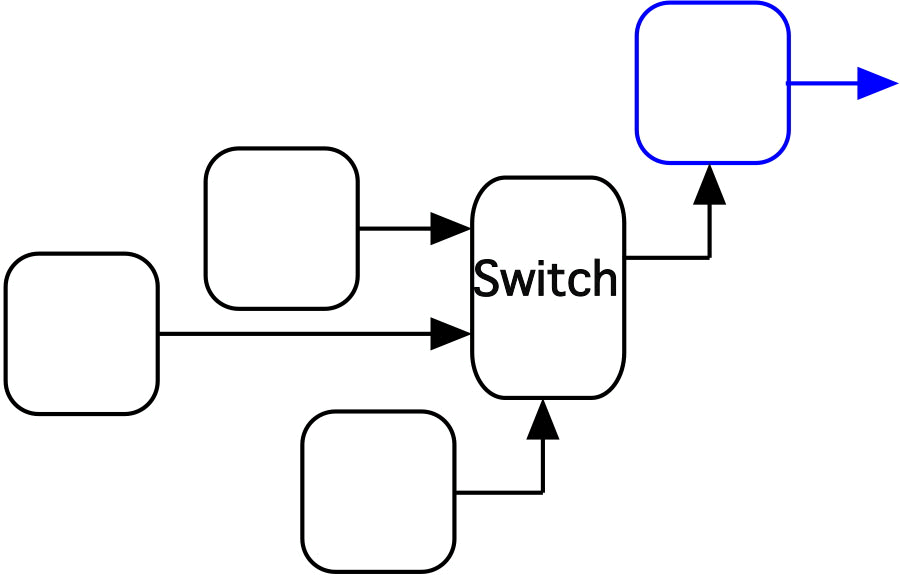
A switch can be added to the control path, thereby providing for two different controls that can be switched (Fig. 50).
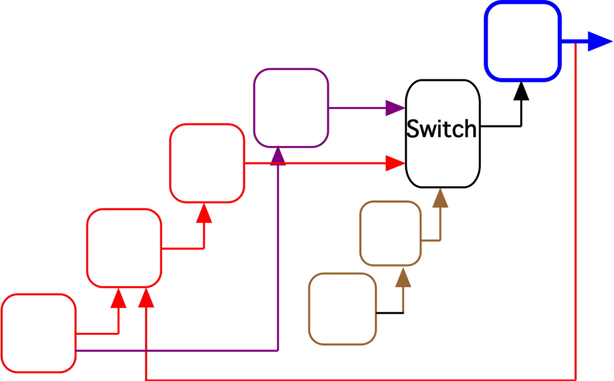
One final example (Fig. 51) includes all of the previous techniques, extended. Set up well, this patch can play itself interestingly for quite a while. The source module (blue) is being controlled by one of two control paths: the three-layer, red path with control from the output to the second layer; and the purple path, which is also being controlled by a module in the red path. The rate of the switching, the clock, is being modulated by a second layer.
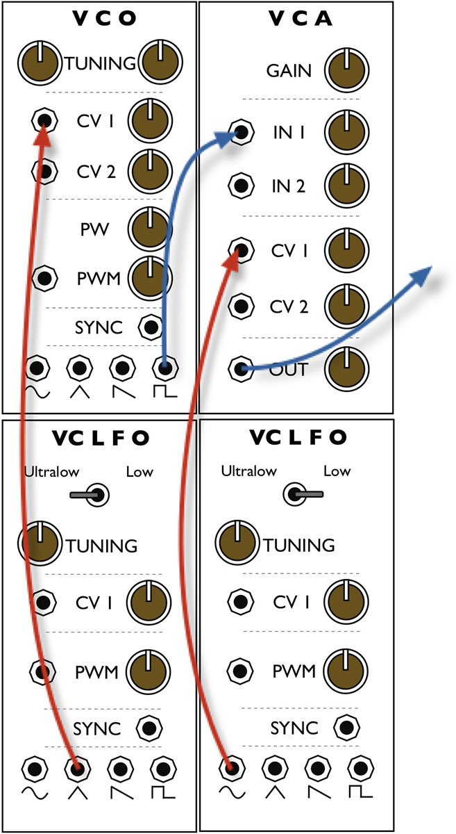
How to Draw a Block Diagramme of a Patch
After creating a complex patch, you may want to document it, both as a patching diagramme and a block diagramme. For the patching diagramme, the best way is to start by taking pictures with your cell phone. As you prepare the block diagramme, you may find it useful to take more pictures.
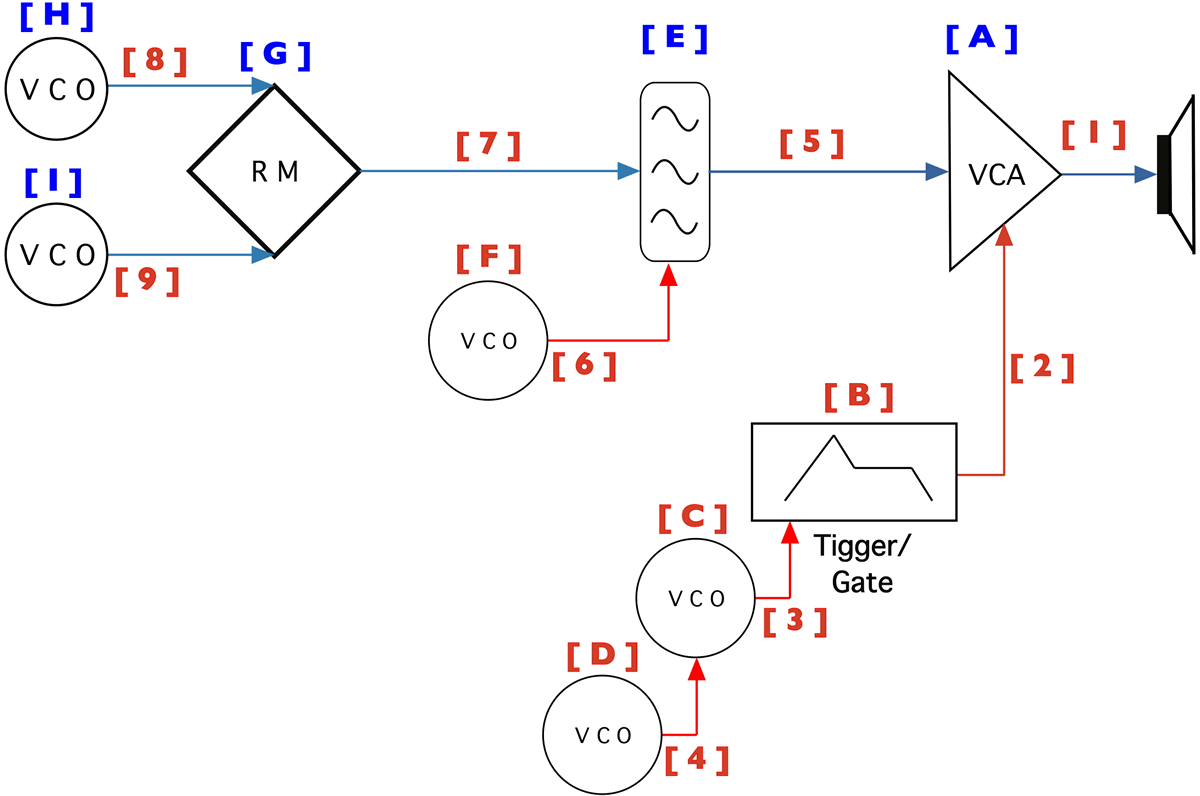
Below is a detailed step-by-step example of the process to follow. Certain conventions have been employed: signal paths are in blue and control paths are in red. The modules have been indicated A through I.
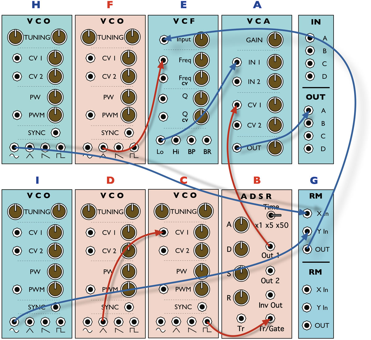
Examine the patch and count the number and type of modules. Note that there are 9 modules in total — 5 oscillators, 1 amplifier, 1 filter, 1 ADSR, 1 ring modulator — and an output.
To convert the patch into a block diagramme:
1) Take a picture (or two) of the patch.
2) Examine the patch and consider how to work backwards from the final output(s). (Keep in mind that if there is more than one output in your patch, there may be several block diagrammes needed.)
3) Start from the output: draw an output module on the far right of the page.
4) Trace the cable back to the previous module, from the OUT A to module A, the VCA output.
5) Draw module A, the VCA and add the line for the patch cable (Fig. 53, 1).
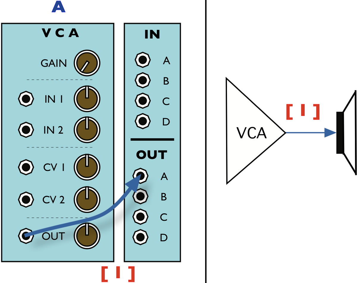
6) Remove the patch cable from the module.
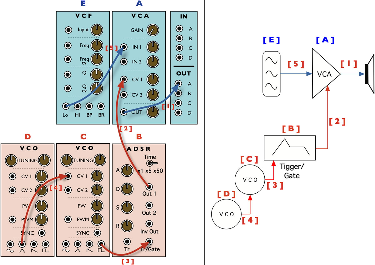
4a) Trace the CV cable from the ADSR to CV 1 input on the VCA.
5a) Draw module B, the ADSR and add the line for the patch cable (Fig. 54, 2).

6a) Remove the patch cable from the module.
4b) Trace a cable from VCO C to the Trigger/Gate input on the ADSR.
5b) Draw module C, VCO C and add the line for the patch cable (Fig. 44, 3).
6b) Remove the patch cable from the module.
4c) Trace the CV cable from VCO D to CV 1 input on the VCO C.
5c) Draw module D, VCO D and add the line for the patch cable (Fig. 44, 4).
6c) Remove the patch cable from the module.
Return to the (audio) signal path.
4c) Trace the cable from the VCF low-pass out, to IN 1 on the VCA.
5c) Draw module E, VCF and add the line for the patch cable (Fig. 44, 5).
6c) Remove the patch cable from the module.
Continue this process until all nine modules and all nine patch cables have been drawn. As much as possible, keep the signal path left-to-right and controls from below.
Module Layout
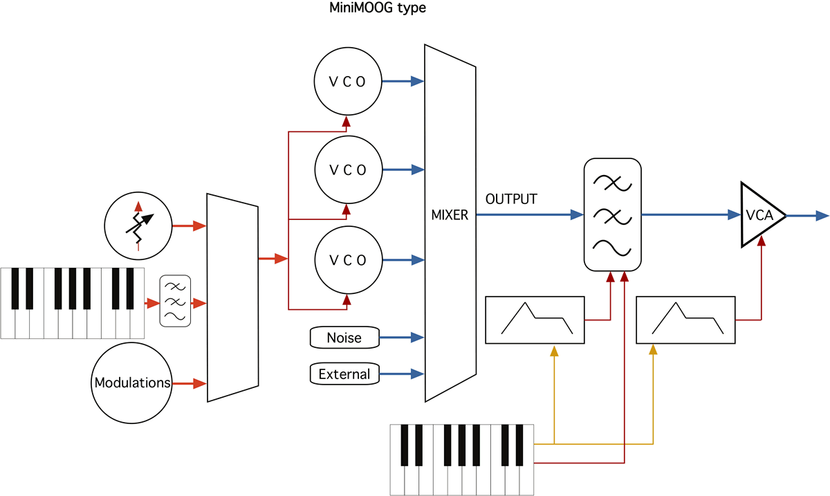
This may not be a serious issue with a small system that is set up with, from left to right, sources, processors and output. This is the “classic” fixed architecture monophonic synth layout from the 1970s and early 1980s (Fig. 57). Limited to about 8–12 “modules”, generally these synths did not use patch cables and the limited routing was established by the use of switches. There were few “logic module” options and they were treated as controls.
With systems that are between 20 and 50 modules, a number of decisions need to be taken for the layout. The “random” option is possible, but learning the layout and modifying the layout design becomes difficult. With 60 to 120 modules, other possibilities emerge.
Instrument Model
One model of an acoustic instrument is seen in Figure 58. The energy “source” is followed by processes of filtering. A gong is struck. The impulse sets the piece of metal into random vibration. The shape and size of the gong filters out frequencies that do not resonate. The energy dissipates over time. Some instruments have controls on these two processes, for example a guitar string can be longer or shorter, could slide between states and the processes could include damping, filtering, feedback, etc.
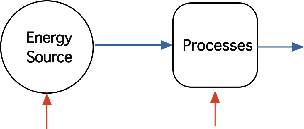
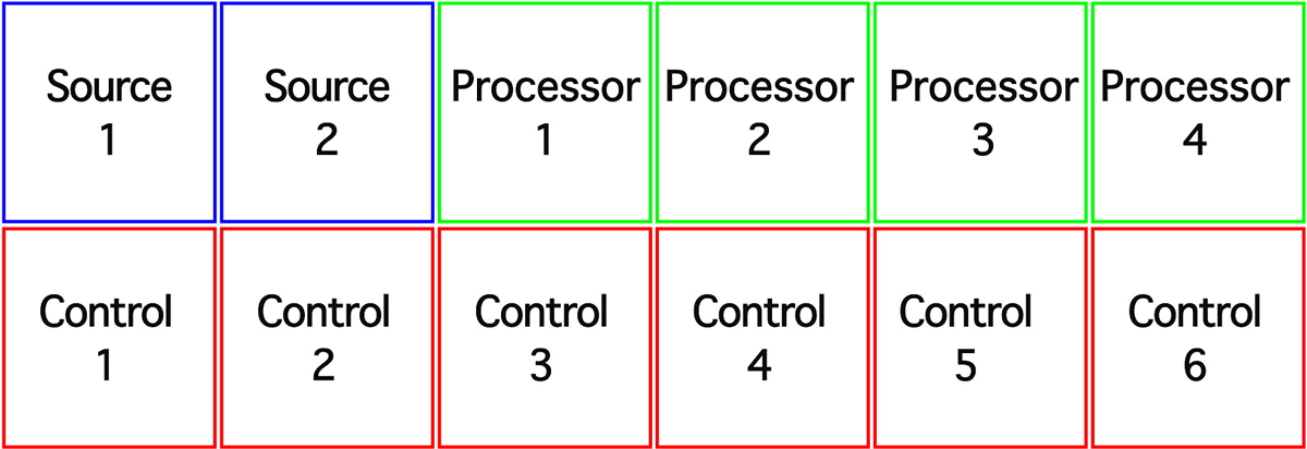
Module layout for a modular system based on this model would place the sources to the left and a daisy chain of processors to the right, with controls below (Fig. 59).
This is the standard design, with (left to right) sources going into processors and controls fixed below, of a small, basic keyboard synth as described above. Often there will be some routing options and shared control modules, such as LFOs. Putting these 12 modules into a rack would look like Figure 60.
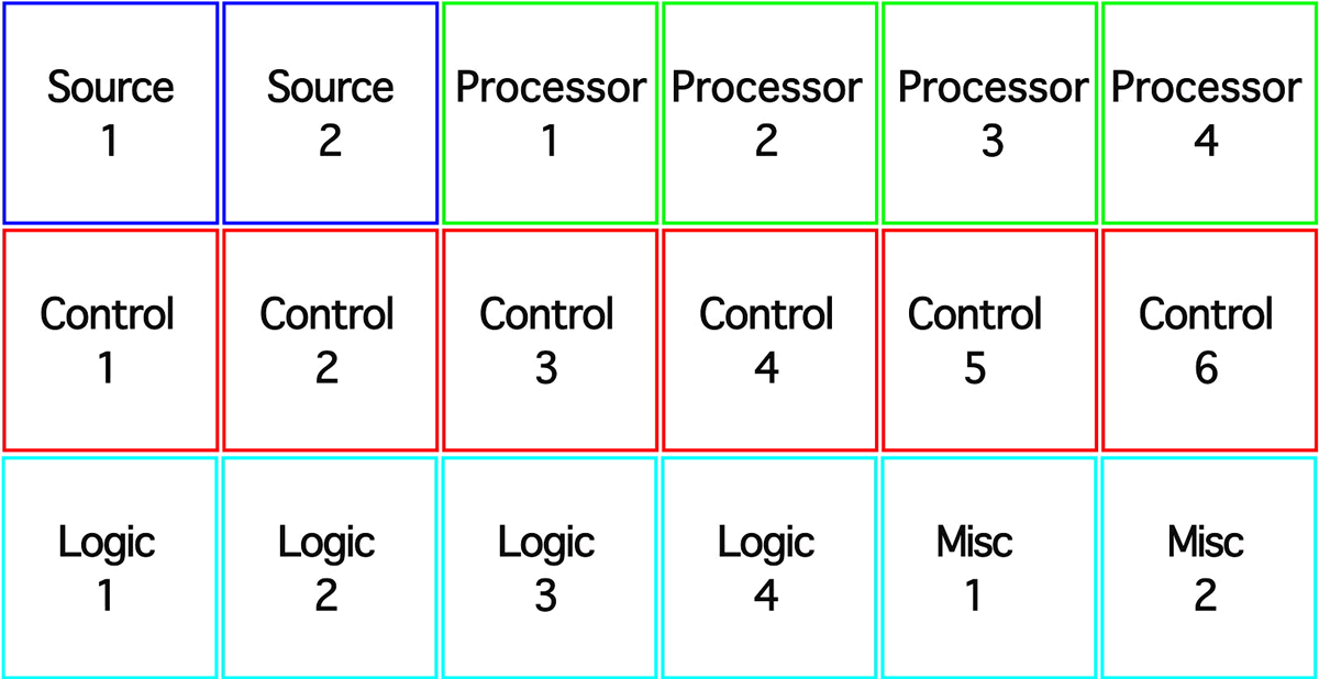
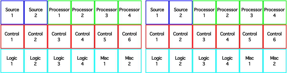
With the addition of logic and miscellaneous modules, a basic “instrument” is available (Fig. 61).
A doubling of the number of modules could produce two instruments (Fig. 62).
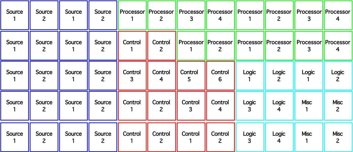
Another approach is to cluster all related types of modules together so that, for example, all of the oscillators are together in one area, all of the filters are together, amplifiers, etc. (Fig. 63). This design approach is useful for large patches as it is easier to find “another” ADSR when they are all together in one place!
Postlude
The modular synthesizer allows the user to set and vary sonic parameters independently. That is, the frequency, amplitude, spectrum etc., can be created and modified without interacting with each other.
This Generalized Introduction to Modular Analogue Synthesis Concepts is based on materials built up starting in the early 1970s when a course on Electronic Music was given at Sir George Williams University, subsequently Concordia University in Montréal, Canada. Initial notes were prepared for classes explaining the modules and functions of the Synthi AKS that was in the studio at that time.
The purchase of an Aries system in 1978 introduced a modular synthesizer with about 45 modules. Documentation that was prepared for this system included practical aspects of how each module appeared and how to patch modules together, along with some fundamentals of modular synthesis. The Aries slowly disintegrated and in 2009 was replaced by a 90+ module system from Doepfer.
The original documentation prepared for the Aries by Kevin Austin ca. 1977–2005, with additional contributions by Mark Corwin, was adapted and modified by Paul Scriver in 2009 and has been significantly updated as a guide to the whole system in 2011–12. Additions appeared in 2013, 2014 and 2015.
The Concordia University Doepfer system is (in 2016) in four independent road cases. The two taller cases are about 80% similar in content and layout. Using the “instrument model” (Fig. 58), the top left corner contains the source modules — VCOs and noise sources, the end of the top row and part of the second row contain processors, the remainder of the second row contains control function modules and the bottom row contains control and logic functioning modules (Fig. 64). They are referred to as “voices”.
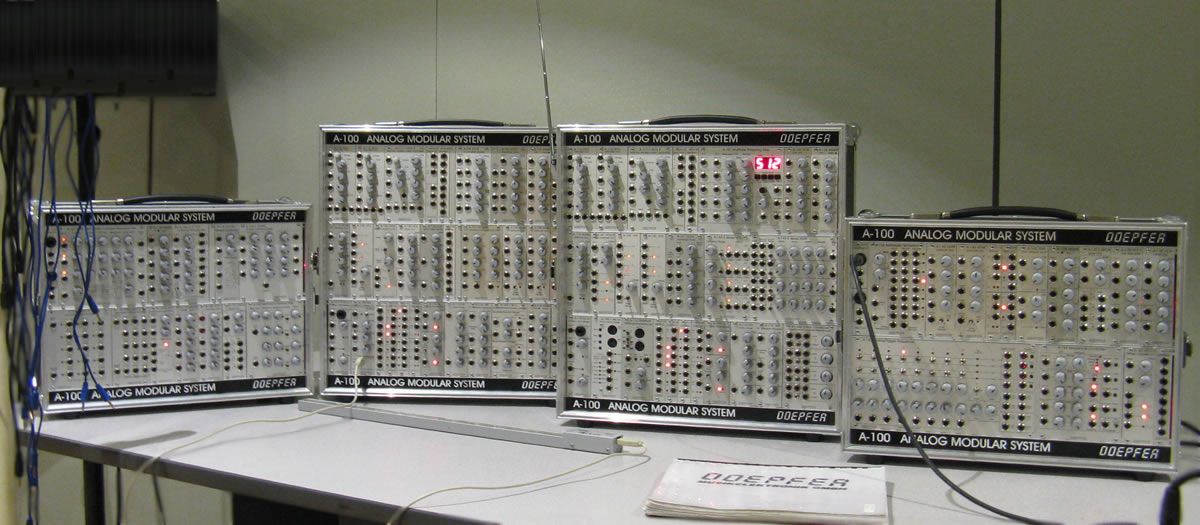
The left side case has a vocoder in the bottom left and spectrum / waveshaping modules. The right case has a step sequencer and mostly logic modules. It has been designed to allow up to four people to play at the same time, with the two-voice cases and the left-side case being used for external processing, and the right-side case for sequencer and logic patches.
Article Content, References and Citations
This article grew out of a need to bring together modular analogue synthesis concepts succinctly into one place. It is related to the documentary guide to the analogue synthesizer modules found in modular system at Concordia University in Montreal, prepared by Kevin Austin, with additional materials provided by Mark Corwin, Paul Scriver and Eldad Tsabary, and others from the period 1975–2015.
I would like to thank the hundreds of students who have provided comments on how to learn modular analogue synthesis and the half dozen or so instructors who have added thoughts or even prepared revisions for the course materials.
For the sake of limiting the article from becoming a general introduction, there is a certain amount of brevity in explaining / defining many concepts. Some readers may need to consult secondary sources if certain basic concepts are not known or understood. There are hundreds of sources for this information and in general the best approach is to Google any terms that are not clear.
Addendum: Later Thoughts on Simple and Compound Modules
In response to a question about an octave equalizer in about 1970, Hugh Le Caine passed on the comment, “It’s all only amplitude,” or something very similar. In my mind I add the extension, “ — anyway.” I had taught myself basic analogue synthesis before I had learned much about electronics or psychoacoustics, and while I kind of understood what he meant, the actual depth of the comment eluded me for a while.
The model is this:
- The ear drum is displaced by a soundwave. It can only have one displacement at any moment in time.
- The cone of a loudspeaker is displaced by a voltage. It can have only one displacement at any moment in time.
A deep consequence of this is that the only (actual) parameter of sound (as acoustical energy), is amplitude. The only “simple” module, is, ipso facto, an amplifier. The amplifier has an output that is a function of the control of the amplitude of its input. Beyond the amplifier, the simplest module is noise — which is random. A random control, in this case molecular noise, is multiplied by the amplifier to produce an output level that is required by the system.
An oscillator is an amplifier controlled by a cyclical event sequence. The simplest oscillator would have a control that switches from low to high. This transition can be sudden, producing a pulse wave. Or, for example, it could be an increasing level that at its peak returns immediately to the zero state — a sawtooth wave. In terms of the model, this is already a “compound” module, being an amplifier and a control circuit.
The essence of the circuit is not the signal path, but rather the design and implementation of the controls and control path. It is possible, for example, to design a module which is an amplifier, the output of which is being controlled by a 100-stage sequencer, running at, for example 4.8 MHz — the sampling rate for one hundred 48 kHz signals, each of the one hundred steps being independently controlled. This is at the core of the Razor module made by Native Instruments. This is not additive synthesis, as additive synthesis requires a mixer to add the signal path voltages together. It is a form of “non-interactive multiplex synthesis.
A second(ary) deep consequence of this model is that frequency is not inherent in the primary signal. It is an applied control, and also, in perception, its decoding occurs in the brain. Similarly, spectrum doesn’t exist in the signal, but is a psychoacoustic attribute. This extends to the concept of sound object, object recognition, transformations, etc.
Seen historically, this particular path of thought was pursued most rigorously in Germany by Karlheinz Stockhausen, and in the United States in computer music research.
Social top